< Back to A Level Cheat Sheets
OCR A Level Geography - COMPLETE Paper 1 (Physical) Revision Notes
⚠ Please note, this is a work-in-progress, somewhat unfinished document. The most unfinished sections are marked with [tbd] and there may be general issues and typos. ⚠
Latest update: 12/05/2025 19:55.
Last content addition: 07/06/2024 22:18.
✅ Note: This file is synced with this repository. This is the latest version.
Use a PC/device with a large screen to see the Table of Contents on the left-hand side to quickly navigate through this document.
Discuss with other students, developers, educators and professionals in the Baguette Brigade Discord server! You can also receive a notification when there are new Cheat Sheets, Summary Sheets (new!) or other revision material is made public there!
For the Cheat Sheet matched to the entire specification, you can go here.
Glaciated Landscapes
“Feeling a little like a drumlin today.”
Check out this interactive BRITICE glacial map to see places in the UK which have been influenced by glacial activity, with drumlins, subglacial lineations, moraines and more, from Sheffield University!
Glaciers as Systems
1.a. Glaciated landscapes can be viewed as systems.
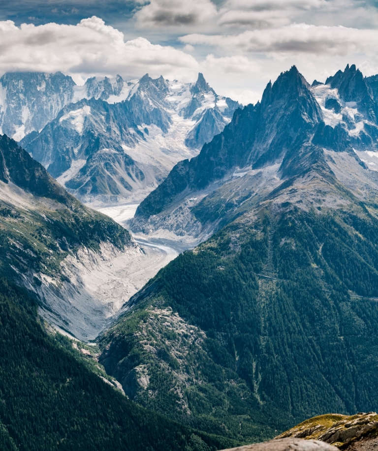
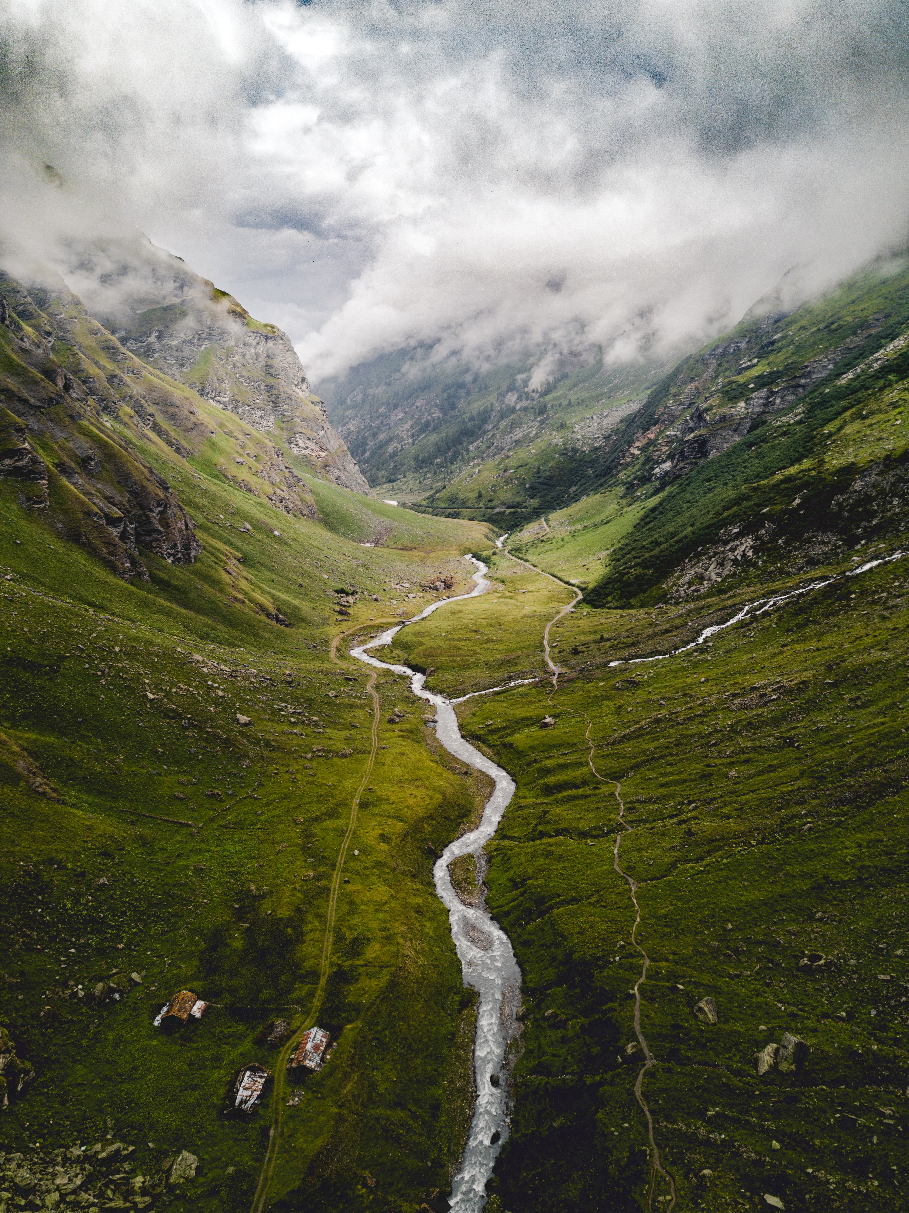
Valley glacier photo from Simon Fitall.
There are 3 main parts to any system: inputs, processes and outputs.
Glaciers are dynamic. Glaciated landscapes may be seen as a system with many interrelated components (stores), processes (cause/effect mechanisms), inputs and outputs. This forms an open system.
- Inputs
- precipitation (snowfall)
- material from deposition, weathering and mass movement
- avalanches
- thermal energy (from the sun)
- kinetic energy
- Outputs (Ablation)
- evaporation
- sublimation
- wind erosion
- meltwater
- Stores
- ice
- water
- debris
- potential energy (from its location)
- Throughputs/processes
- debris movement downslope
- deposition
- kinetic energy from glacier movement
Glaciers themselves can be seen as systems as they have a TON of different inputs, outputs, flows (or transfers) and stores.
Useful key terms
- Terminus - the end of a glacier
- Snout - the end area of a glacier
- Ablation - melting
- Calving - when chunks of a glacier terminus fall into water
- Advance - when a glacier is moving forwards; gaining mass balance
- Recession - when a glacier is retreating; losing mass balance
- Area of accumulation - the area of a glacier where it is gaining mass
- Area of ablation/wastage - the area of a glacier where it loses mass
- Névé - young, granular snow
- Firn - névé which has survived a full season (year) of ablation and is partially compacted, and has been recrystallised into a substance denser than névé, an intermediate stage to becoming glacial ice.
- Firn line/equilibrium line - the zone on a glacier where accumulation is equal to ablation over a 1-year period
- Sintering - continued fusion and removal of air as a result of compression by the continued accumulation of snow and ice
- Aspect - the direction that a slope faces.
- Azimuth - the compass direction of an object
The Glacial Budget and Mass Balance
A glacier forms when snowfall exceeds summer melt in an area, resulting in the accumulation of snow and ice year after year, typically in a hollow on a mountain with a northwest-southeast aspect in the northern hemisphere.
Over time, snow is compacted and turned into glacial ice, and when this is around 40m thick, the intense pressure causes it to begin flowing. The top of the glacier is white, but glacial ice at the base of the glacier is blue as oxygen has left the system.
Snowflakes -> Granular snow -> Névé -> Firn -> Glacial ice
Glacial ice has a density of 850kg/m3. It is rock hard, feels glassy and is almost translucent.
The glacier mass balance is the total sum of all the accumulation (snow, ice, freezing rain) and melt or ice loss (from calving icebergs, melting, sublimation) across the entire glacier, or amount of ablation.
Over a year, the graph of mass balance in a northern hemisphere glacier may look like this in a typical scenario:
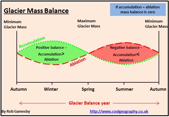
An equilibrium is reached between accumulation and ablation are equal. This point may be reached between the accumulation extreme in winter and the ablation extreme in the summer season. In the image above, as the accumulation is equal to ablation, the glacier is not growing.
Layers of snow within the ice give evidence of the way that it has formed.
Types of glacier and movement
(Date studied: ~29/09/2022)
An ice sheet is a mass of snow and ice, greater than 50,000km2 with considerable thickness.
A piedmont glacier spreads out as a wide lobe as it enters a wider plain typically from a smaller valley
A valley glacier is one bound by valley walls, coming from a higher mountain region, from a plateau on an ice cap or an ice sheet.
An ice cap is a dome-shaped mass of glacial ice usually situated on a highland area and also covers >50,000km2.
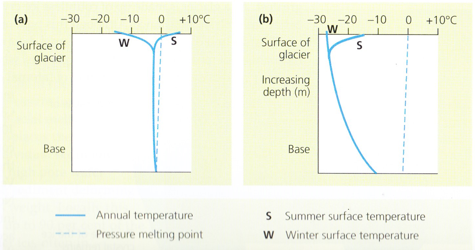
Cold-based (polar) glaciers:
- have a slow rate of movement (<5m/year);
- are located in extreme latitude (polar) regions;
- are generally flat;
- have a low basal temperature, remaining stuck to the bedrock below the pressure melting point;
- are formed in low precipitation areas, and the glacier remains below freezing point during all seasons.
Warm-based (alpine) glaciers:
- have rapid movement (20-200m/year);
- are located in high-altitude (mountainous) regions;
- have a basal temperature at or above the pressure melting point;
- are in areas of steep(er) relief;
- have water present throughout, with the ice acting as a lubricant.
Cold-based glaciers are unable to move by basal sliding as the basal temperature is below the pressure melting point. Instead, they move through internal deformation.
Ice at 0°C deforms 100 times faster than at -20°C. Thus, the movement within cold-based glaciers is limited by there being a lack of lubricant, and the cold temperatures inhibiting internal deformation to a very slow rate.
Factors affecting the microclimate
The microclimate is a small region with its own distinct climatic characteristics, for example, one side of a mountain, or the north side of a valley. Generally, wider climate characteristics play a larger role in influencing the behaviour of glaciers, but glaciers are also affected by various lower-level and smaller-scale conditions.
Relief and aspect
These have an impact on the the microclimate. This is a small region with its own distinct climatic chawalls**, coming from a higher mountain region, from a plateau on an ice cap or an ice sheet.
Valley glaciers usually occur in high altitude locations, with high relief, have fast rates of flow at 20–200m/year (mostly warm-based) and have distinct areas of ablation and accumulation, descending from mountains.
Ice sheets, however, are large masses of snow and ice defined by being greater than 50,000 km² and are usually in locations of high/low latitude and have slow rates of movement of only around 5m/year (mostly cold-based). The base of the glacier is frozen to the bedrock and has a little precipitation but also lower temperatures so ablation levels are lower too.
Fundamentally, glaciers move because of gravity. The gradient influences the effect of gravity on glaciers - areas of high relief mean there is greater gravitational potential energy for faster glacial movement. The thickness of the ice and the pressure exerted on the bedrock can also influence melting and movement. More accumulation also leads to more movement. When ice is solid and rigid, it breaks into crevasses (big gaps visible from the surface). Under pressure, ice will deform and behave like plastic (in the zone of Plastic Flow on the lower half of the glacier) making it move faster. Conversely, the rigid zone is on the top half of the glacier.
Regional climate
The wind is a moving force and can carry out processes such as transportation, position and erosion. In the air, these are known as aeolian processes, and can contribute to shaping glaciated landscapes. It is more effective when acting upon fine materials - usually those previously deposited by ice or meltwater - such as smaller rocks, dirt and sand.
Temperature within the climate is another factor, as temperatures above 0°C will melt accumulated snow and ice, resulting in more outputs in the system. At higher altitudes, there are typically more prolonged periods of above-freezing temperatures, and melting, compared to in high latitude locations, where is below freezing most of the time, allowing for glaciers to thicken and expansive ice sheets to form. Precipitation is another climate factor, with its totals and patterns, both regionally and seasonally, in determining the mass balance of a glacier system, as it provides the main inputs to these glaciers as snowfall.
Latitude and Altitude
Beyond the Arctic and Antarctic circles, located at 66.5° north and south, the climate is very dry, with little seasonal variation. Being so dry and extremely cold, they are much different to more dynamic valley glaciers as they have higher precipitation levels, and more névé turns into firn. The dryness contributes to periglacial environments (see below for more about those!) while also turning the types of glaciers in these areas to more cold-based. This means that they flow much less quickly, and different types of movement occur.
Altitude also has a direct impact on the temperatures and development of valley glaciers. As temperatures typically decrease by 0.7oC every 100m of altitude gained, there are more likely to be valley glaciers in areas of high relief, as seen in the Alps and the Himalayas. These glaciers are still not as cold as cold-based glaciers, however.
Geology
Geology is more than just “weak” and “strong” rocks and resistance. It is a combination of properties that uniquely determine how rocks react to stress, mechanical and chemical forces, and the environnment.
Lithology is the chemical composition and physical properties of rocks. Some types, like basalt, are very resistant to erosion and weathering, as they are comprised of densely packed interlocking crystals. Clay, on the other hand, is weak and does not have these strong bonds on the molecular level. The solubility of rocks like chalk can also be affected by acidity, making them prone to chemical weathering, as seen through carbonation. Weakly-bonded rocks also reduce their resistance to glacial erosion.
Structure relates to the physical rock types, like faulting, bedding and jointing. These all have an impact on how permeable rocks are. Chalk, for example, is very porous, spaces between the particles within it on the molecular level allow water to percolate through. In glaciated environments, this is significant as freeze-thaw action can crack rocks with faults or pores from the inside. This compares to crystalline rocks such as igneous granite which do not have any of these structural weaknesses.
Some types of limestone, like carboniferous limestone, have many interconnected joints, giving it ‘secondary permeability’.
Primary permeability is when spaces (pores) absorb and retain water.
How are glacial landscapes developed?
Glacial landforms are typically classified according to erosional and depositional processes. This development can be described as a series of interrelated processes.
Glacial erosional landforms
Corries
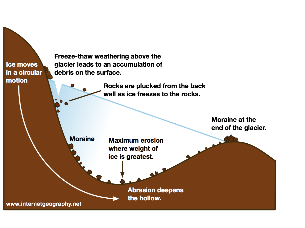
The processes occurring in a corrie.
A corrie is an armchair-shaped depression in a mountain. Also known as a cwm or cirque, they are formed from small hollows on the slopes of mountains where snow begins to accumulate, typically on the north-west to south-east facing slopes (or with an azimuth ranging from 300-140 degrees) on a mountain in the northern hemisphere.
This is due to its aspect, or the orientation of which a slope faces, with this specific aspect resulting in having less insolation. Greater amounts of irradiation add thermal energy to the system, resulting in ablation.
This virgin snow is known as névé, which becomes firn after one complete cycle without melting (i.e. surviving a summer ablation period; of 1 year).
This newly-formed hollow, deepened by nivation (e.g. freeze-thaw processes) from the ice, then begins to move because of gravity acting upon the ice mass. The ice freezes to the back wall, plucking material (debris), which is then washed out through a process known as rotational slipping. Over multiple years, the snow at the bottom is compressed into ice, and the material plucked or that has fallen into the bergschrund crevasse is used by the ice to abrade and further deepen the hollow. Comparatively, the ice at the front of the corrie may be much thinner and therefore has lower pressure and is less abrasive, creating a rock lip, supplemented by washed out moraine from previously plucked material.
When this ice melts or the area is deglaciated, a tarn (or corrie lake) is created, enclosed by the rock lip. Material may then continue to fall down from the back wall due to continued weathering, combined with aspect and steep relief, known as scree.
Arêtes
An arête is a knife-shaped, narrow ridge formed when two corries’ back walls continually erode back-to-back. Over time, these back walls meet, and a distinct ridge is formed.
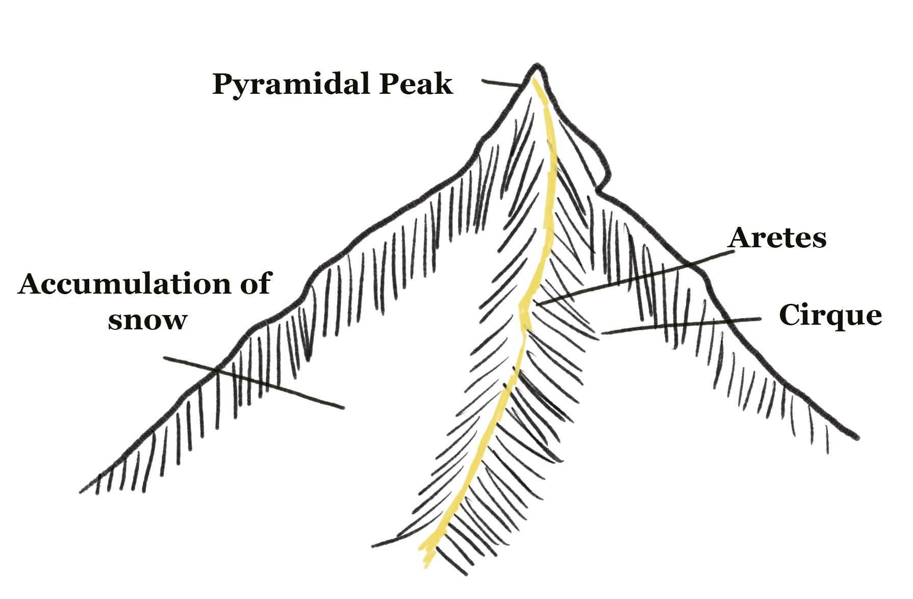
A diagram of a mountain, which has had erosional processes acting upon it.
Pyramidal peaks
A pyramidal peak is a high mountain whose surroundings have been eroded as corries. Three or more corries eroding back-to-back (similarly to how arêtes form) result in this sharp peak forming. There are typically distinct aretes visible all the way up to the peak, representing the boundary between corries.
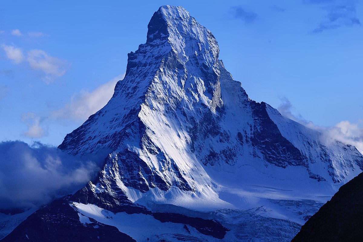
The Matterhorn in the European Alps. It is a great example of a pyramidal peak.
U-shaped valleys
Also known as a glacial trough, a U-shaped valley is formed as a result of strongly channelled ice, bulldozing its way through a valley. On the valley’s sides, plucking occurs, causing the sides to steepen. This rocky material is then dragged by the glacier, helping it to carve out more of the landscape.
The actual shape of most U-shaped valleys is parabolic.
Firstly, before a glacial period, a V-shaped valley exists, having moderately steep sides and a central river channel, with interlocking spurs being a distinct feature. During periods of glaciation, snow begins to accumulate in these valleys as they are often sheltered.
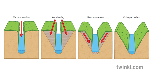
How a V-shaped valley is formed. Remember this from GCSE? (if not, recap yourself on the GCSE Geography cheat sheet!
When an ice mass has formed in the valley or has flowed from an upland area, freeze-thaw weathering begins to occur above the glacier line (where this ice mass is), causing the valley to steepen, in the same way as a corrie steepens its back wall. The glacier itself also causes plucking, mostly on the sides, as rocks are frozen and ripped as the glacier moves. Vertical abrasion also deepens the valley floor as subglacial material comes into contact with the bedrock.
Hanging valley
Hanging valleys with waterfalls and truncated spurs are a feature of the U-shaped valley landform. They are visible within this glacial trough, and form as a smaller glacier from another valley has created a U-shaped valley which then enters the larger valley. As the hanging valley’s glacier is smaller, it is less powerful, so it does not reach the base of the larger glacial trough valley.
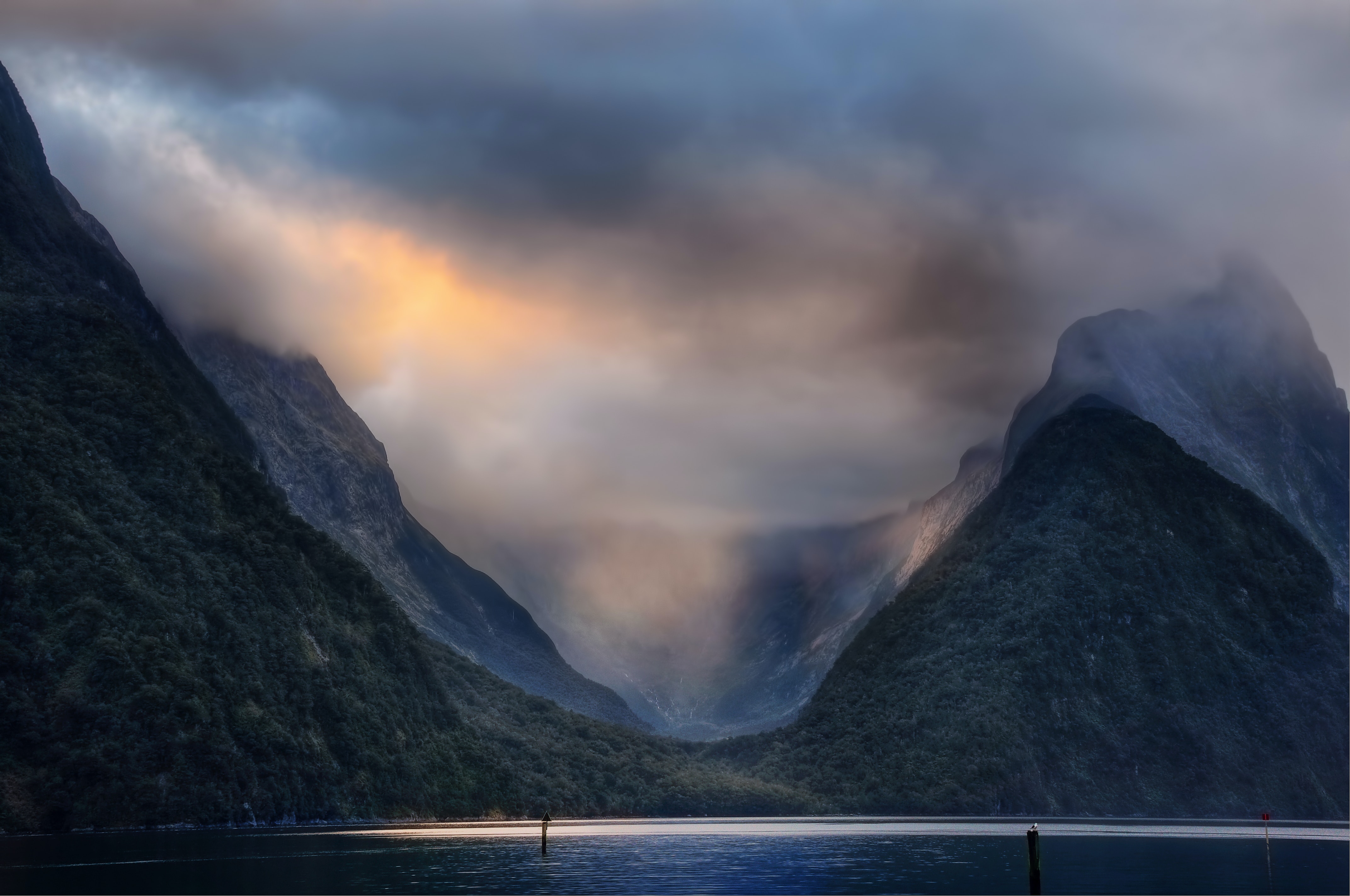
Photo from Peter Hammer.
Water features
After deglaciation, there may be some (iconic) water features in these glacial troughs.
Ribbon lake
Glaciers erode the valley into the typical U-shape. These lakes are typically long, thin and deep as a result of compressing flow, as this ice is likely to have come from an area of high incline to a more expansive area. This means that the ice is more likely to move faster and pushed into a thinner area downstream, so is more likely to erode vertically rather than laterally. This depression (or rock basin) is then refilled with water after a glacier retreats. More detail over at Ullswater in the Lake District case study section.
Misfit stream
A ribbon lake and a misfit stream may also be present in the base of the newly-formed glacial trough valley after deglaciation.
Misfit stream: Photo from Mario Álvarez.
Roche moutonnées
A roche moutonnée is a more resistant rock in the path of a glacier. Light abrasion from the above subglacial material occurs on the upvalley (stoss) side, resulting in striations, grooves, and polishing from subglacial debris. There may also be pressure melting at a local scale on this side.
As this meltwater is forced up and over the roche moutonnée, mechanical plucking and freeze-thaw weathering occur. On the down-valley (lee) side, the pressure release results in refreezing into ice, while the glacier continues to move, thereby pulling away the rock and giving it a craggy appearance.
Roche moutonnées are generally concentrated in areas of competent bedrock, such as granitoids (Glasser, 2002) - this essentially means that rocks are somewhat resistant to deformation.
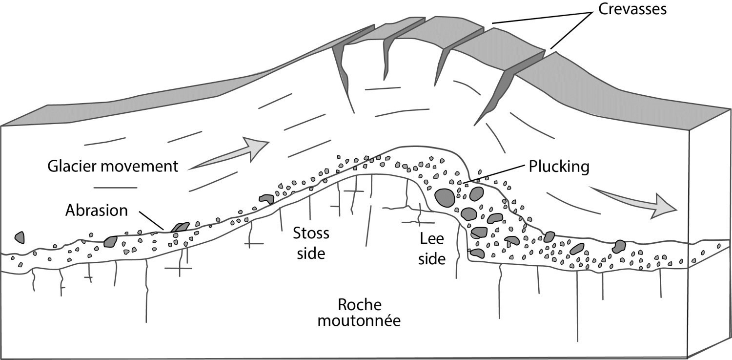
Source: Québec government website
The word is French with “roche” meaning rock and “moutonée” meaning sheep.
More specifically, it was introduced by a French geologist called Horace-Bénédict de Saussure (1740-1799). The word is called like so due to its resemblance to the shape of a wig, worn by 18th-century French aristocrats which shaped their hair like a wave. Sheep fat was used to hold the wig in place, which explains the term moutonné (Benn and Evans, 2010). In Sweden, very large roches moutonnées are called flyggbergs, with some being up to 3 km long and 350 m wide (Rudberg, 1954; 1973; Iverson et al., 1995; Benn and Evans, 2010).
Ellipsoidal basins
These are no ordinary valley or alpine glacier erosional landform. These are huge areas formed by ice sheets such as the Laurentide Ice Sheet in North America. (more detail with the Minnesota Ice Sheet Case Study)
These huge ice sheets (more than 50,000km2) exert large amounts of pressure on the landscape as well as great erosional quarrying by subglacial material. Examples of this feature include Hudson Bay, and smaller ellipsoidal basins created the Great Lakes in North America.
On top of the subglacial erosion which may have occurred, some of this large-scale erosional landscape’s formation is also due to isostatic lowering. This involves the sheer mass of the ice sheet, potentially several kilometres thick, exerting pressure on the lithosphere and effectively compressing it into being smaller.
After deglaciation, isostatic readjustment may occur, and these compressed, lowered areas may readjust and bounce back upwards, now being under no additional pressure.
Glacial depositional landforms
- Supraglacial material is material which is located on the top of a glacier.
- Englacial material is material which is located inside a glacier.
- Subglacial material is material which is located on the base of a glacier.
- Material deposited during glaciation is called drift.
- Material deposited directly by ice is called till.
- Material deposited by meltwater is called outwash, or glacio-fluvial material.
Lodgement till is material deposited by advancing ice, due to pressure being exerted into existing valley material, and left behind as ice advances, such as the theory of depositional drumlins.
Ablation till is material deposited at the terminus by melting ice from stagnant, or retreating glaciers during a warm period or end of glaciation event. Most depositional landforms are this type.
It can be known whether sediment was deposited by water or ice. Ice-transported sediment is angular, not curved, as it has not been subject to more abrasive, erosional forces by the meltwater. The order of size of sediments can indicate this too, as water deposits sediment progressively due to reducing energy levels, while glaciers deposit material unsorted; ‘en masse’. Glaciers also deposit till in mounds and ridges, as, during ablation, this englacial and supraglacial material gets dropped on the bedrock below. This is distinct from the layered deposition (or strata) typically characterised by fluvial processes. Glaciofluvial processes involve an amount of stratification but not complete sorting.
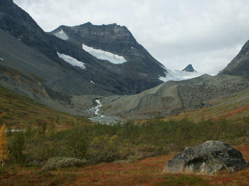
There are a range of depositional landforms visible in this photograph. Can you identify them all?
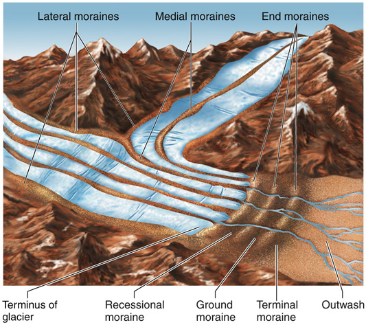
A great diagram of all the different types of moraine.
Moraines
Moraines are ridges of soil, rocks and till which have been deposited by a glacial system. They are added to the glacial system over time through weathering, rockfalls, freeze-thaw action, etc.
Strictly speaking, only the main three are on the OCR specification, but there’s no harm in being able to explain them all.
Medial moraines
Form in the centre of a glacial channel (typically when two glaciers merge - see the image above and you can see how the mountain in the middle is being carved out). Also may occur when their lateral moraines meet and combine into one.
Lateral moraines
Ridges which form on the sides (margins) of a glacial channel, and are the result of the accumulation of debris due to erosional processes on valley sides such as freeze-thaw.
End moraines
These mark a pause or halt of glacial retreat (e.g. when there are a couple of decades with little advance or retreat). These pauses typically are not very long so deposits reflect this, not being too large either (100m max)
Terminal moraine
A ridge, often characterised by being the largest and most prominent in the area, marking the maximum advance of a glacial period (glacial maximum), deposited at the snout of the glacier. Often crescent-shaped when observed from the cross profile.
Recessional moraines
A combination of the end and terminal moraines.
Erratics
They are randomly placed bits of rock and other debris which can be characterised by being of different geology compared to that of surrounding rocks, e.g. limestone in a valley mainly of basalt.
This can be seen in the Lake District where rocks belonging to the rock group Borrowdale Volcanics were found in an area dominated by limestone.
The Bowder Stone is another example being a 2,000-ton andesite lava boulder south of Keswick in the Lake District which most likely originated in Scotland.
Drumlins
Drumlins are unsorted mounds of streamlined till, commonly elongated parallel to the former direction of ice flow, composed of glacial debris.
It is not known exactly how drumlins are formed, but the most likely and agreed upon explanation for their formation is that the glacier becomes overloaded with till (loses competence), so begins to deposit this sediment due to the increased friction that the till brings (‘smearing’ the landscape). This sediment accumulates and quickly compounds, and other till that flows over the initial bump can become stuck, growing this mound of unsorted till. Over time, this grows, and when the glacier retreats, the distinct hill is revealed. This video is a good example of the theory of depositional drumlin formation.
This is an example of lodgement till (not ablation till) as it is formed as the glacier is still advancing.
Others argue that they may have a bedrock core (hence rock-cored drumlins) and as material was obstructed, sediment began accumulating around this, much like in the way of a dune, and was streamlined in the same way as above.
Another argument to the formation of drumlins is that they occur when a glacier move over an area of existing glacial deposits. As the glacier moves over this existing till, the pressure of the overlying ice causes the till to be remoulded and changed into the characteristic shape of streamlined till that we know and love as a drumlin.
They typically occur in larger groups, or ‘swarms’. This is known as a ‘basket of eggs’ topography.
Drumlins can be up to 1,000m in length but are typically around 300-500m. They also improve revenue for farmers, as the topography allows them to have a larger farming area in the same sized plot of land. Their length-to-width ratio is typically between 1.8 and 4.1, and this may be an indication of past glacial velocities, with longer drumlins indicating a faster ice velocity due to the laminar flow of ice.
Drumlins are often found in conjunction with morainic landforms and other depositional features like eskers, kames and outwash plains.
Did you know that the ground between two drumlins is known as a dungeon?
Case study: Lake District
The Lake District is a mountainous area in the north of England. Over the Pleistocene epoch, many glacials and interglacials moulded the area into what it is today, with the most recent activity during the Last Glacial Period (the Loch Lomond Stadial; 12kya) being responsible for the current appearance of the valley landscape.
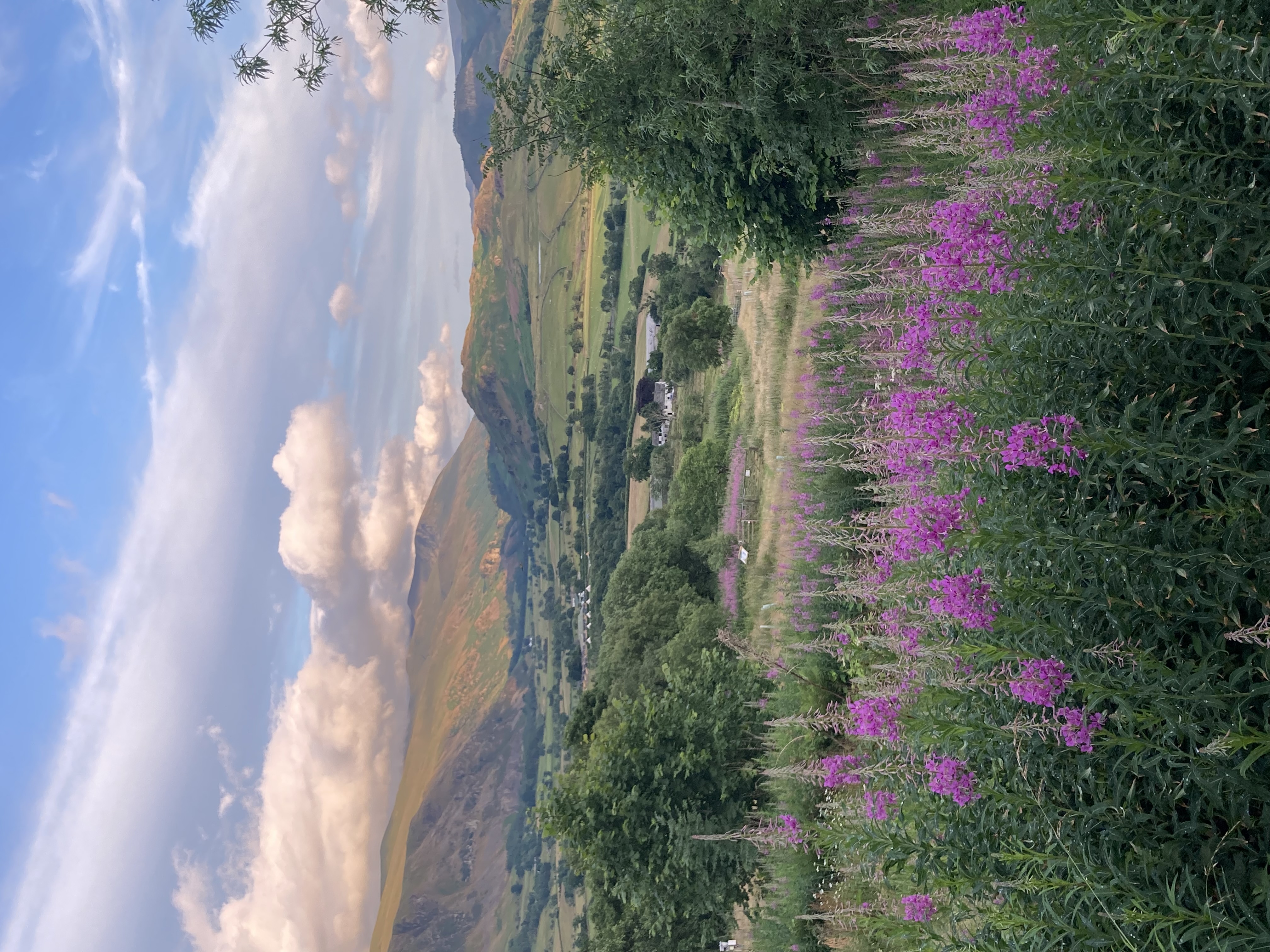
A beautiful view towards Helvellyn from Blencathra.
A range of physical factors have had an influence on the formation of landforms within the landscape.
Geology
The area has three main geologies:
- Skiddaw Group (or Skiddaw Slates - north; the oldest, sedimentary rocks formed 500mya by compaction and tectonic movement)
- Borrowdale Volcanic Group (central; hard igneous rocks formed 450mya including Helvellyn and Scafell Pike (978m) with the largest mountains: it is less prone to erosion)
- Windermere Group (south; softer sedimentary rocks and limestone formed 420mya and have been eroded down)
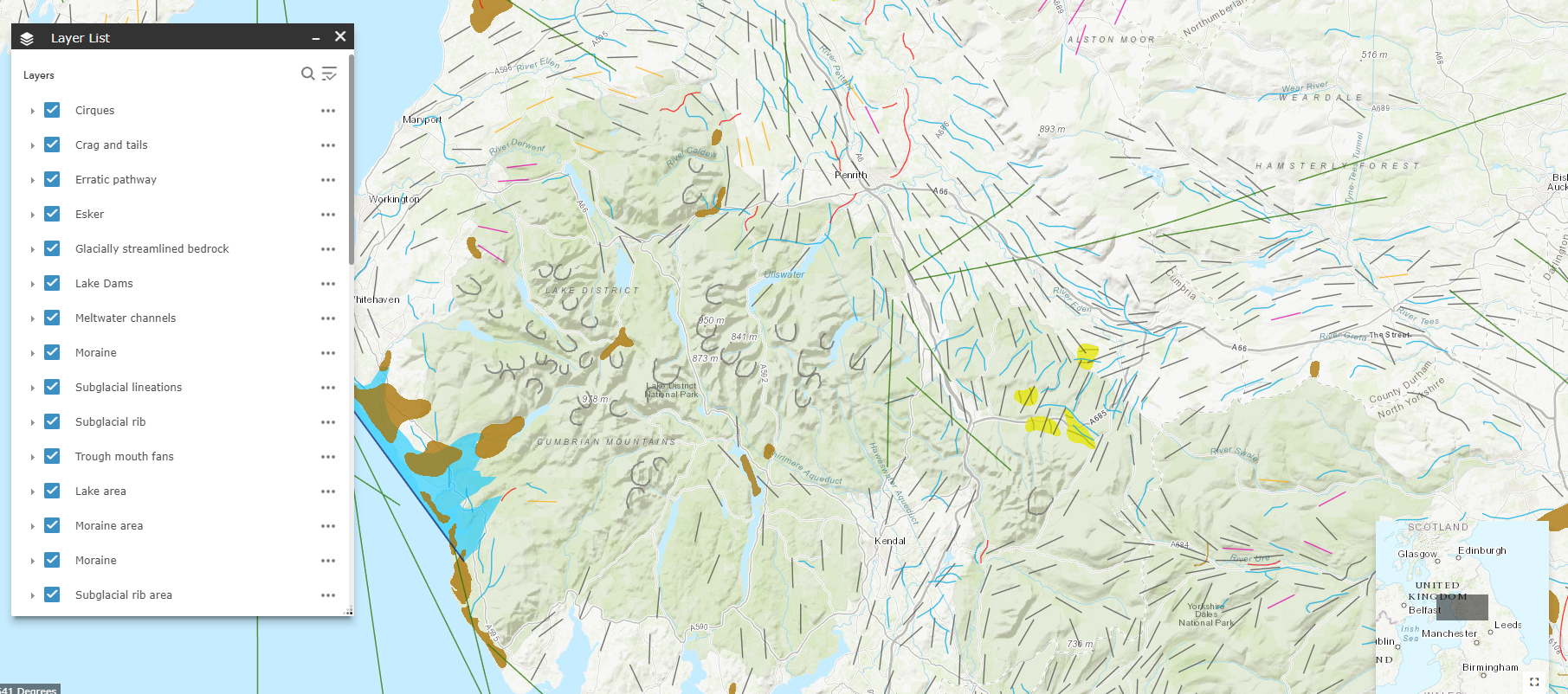
Glacial features of the Lake District, including subglacial lineations, meltwater channels, eskers, drumlins, moraines, glacially streamlined bedrock and more.
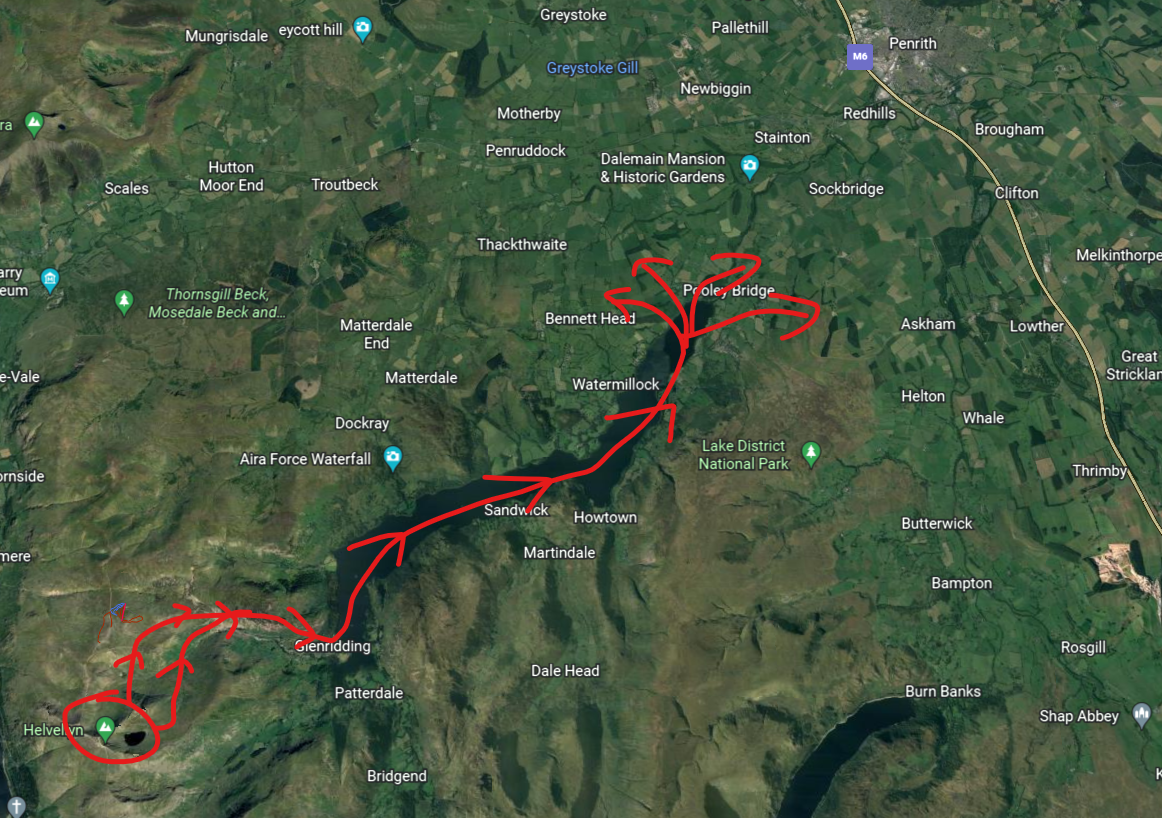
Helvellyn Range
Helvellyn is a 950m tall pseudo-pyramidal peak with aretes named Striding Edge and Swirral Edge separating the corrie from Brown Cove Tarn and Nethermost Cove, respectively. These corries are on the north-east side of the mountain. It’s not quite an official pyramidal peak as it only has these two named corries (but for all intents and purposes…).
Ice from Red Tarn at Helvellyn met with the Brown Cove Tarn ice, creating the Helvellyn Gill hanging valley. Flowing northeast into Glenridding Valley, it joined another larger glacier creating a glacial trough in present-day Ullswater. Likely exacerbated by compressing flow, where the ice mass moves slower, a long, thin, deep ribbon lake formed (as the flow made ice more likely to erode vertically). The varied geology also resulted in extending flow contributing to the ununiformed nature of the U-shaped valley.
This glacier would have continued flowing north-eastwards, taking eroded material with it, towards modern-day Penrith, which is in a flat area, possibly resulting in the old Ullswater glacier becoming a Piedmont glacier when entering this more expansive, larger valley.
Lake District Landforms
Inside modern-day Ullswater is a series of roche moutonnées such as Norfolk Island and Lingy Holm. The geology of roche moutonnées is characterised by being more resistant than other local rock types, possibly with increased jointing and bedding, resulting in striation lines on the stoss, with the freeze-thaw weathering being visible on the lee side still today on these rock islands.
To the west of Helvellyn is the Thilmere ribbon lake. A series of truncated spurs and hanging valleys are located along this U-shaped valley, moulded by a glacier.
Drumlins made of boulder clay have been deposited south of Kendal. They are oriented to the south-west visible here, supporting the idea that the ice was moving outwards from the area of higher topography to lower areas.
Langstrath Valley has an example of lateral moraine on the north side of it.
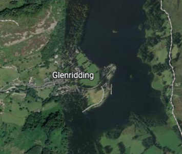
The Glenridding village has visible depositional till extending into Ullswater, visible from satellite imagery, proving that there was once glacial activity in the area.
Essay snippet: inter-related valley landforms
Using a case study, assess the extent to which landforms within a valley glacier are interrelated [16 marks]
Plan
- Formation of corries, aretes and pyramidal peaks: Helvellyn, Red Tarn and Nethermost Cove. Overdeepening caused by nivation, plucking on the back wall, and rotational slip causing the armchair shape - only possible because each are interrelated.
- Back to back erosion w/Nethermost Cove: striding edge arete
- Ice flowing from Red Tarn into Glenridding valley creating Helvellyn Gill and joining with another larger glacier - Ullswater, geologies creating roche moutonnées and deepening of lake. Material from erosion upvalley deposited as sediment visible in the lake today
- Erratics may appear to be not interrelated but from erosion - partly related. Longer distances. Till also forms drumlins typically in flatter areas further away - lodgement till
- Overall, undeniable evidence that all landforms are interrelated through the linked processes of erosion and deposition - with erosion acting as the prerequisite for subsequent transport and deposition.
Essay (note: to rewrite!)
A corrie, or cirque, is formed by snow falling and compacting in a hollow over many winters, typically on the northern side of mountains in the northern hemisphere due to the sheltered aspect, and cooler microclimate. Over time, snow accumulates, compacting the snow beneath it into ice due to the air inside being displaced. The back wall of the mountain, for example, Helvellyn in the Lake District, gets increasingly steep due to persistent freeze-thaw weathering and plucking of material, which then gets entered into the young glacier system as englacial material, or lands on the surface as supraglacial material.
At the same time, under its own weight, the ice at the base begins to rotate, known as rotational slipping, deepening the base through abrasion, with this abrasive material being finer sub-glacial debris. At Helvellyn, the bedrock type is known as the Borrowdale Volcanics, having formed 450 million years ago and moved from tectonic forces. Despite this relative strength due to its more joined and bedded geology, several corries have formed, and their contained glaciers have melted throughout the Pleistocene period. After the most recent glaciation period known as the Loch Lomond Stadial around 12,000 years ago, there exists a corrie containing Red Tarn on Helvellyn’s north-easterly side. These corries have eroded back to back, resulting in the formation of an arête, shaped like a knife, namely Striding Edge, and Swirrell Edge on the alternate side of this corrie. Furthermore, Red Tarn has a lip, helping to prevent water loss, as a result of rock and moraine deposits left by the glacier.
These examples clearly show the significant extent to which landforms in a valley glacier system are interrelated between different erosional landforms, from the initial snowflakes settling in a hollow to the creation of many other landforms during and after glaciation has occurred.
Ice Sheet Case Study: Minnesota
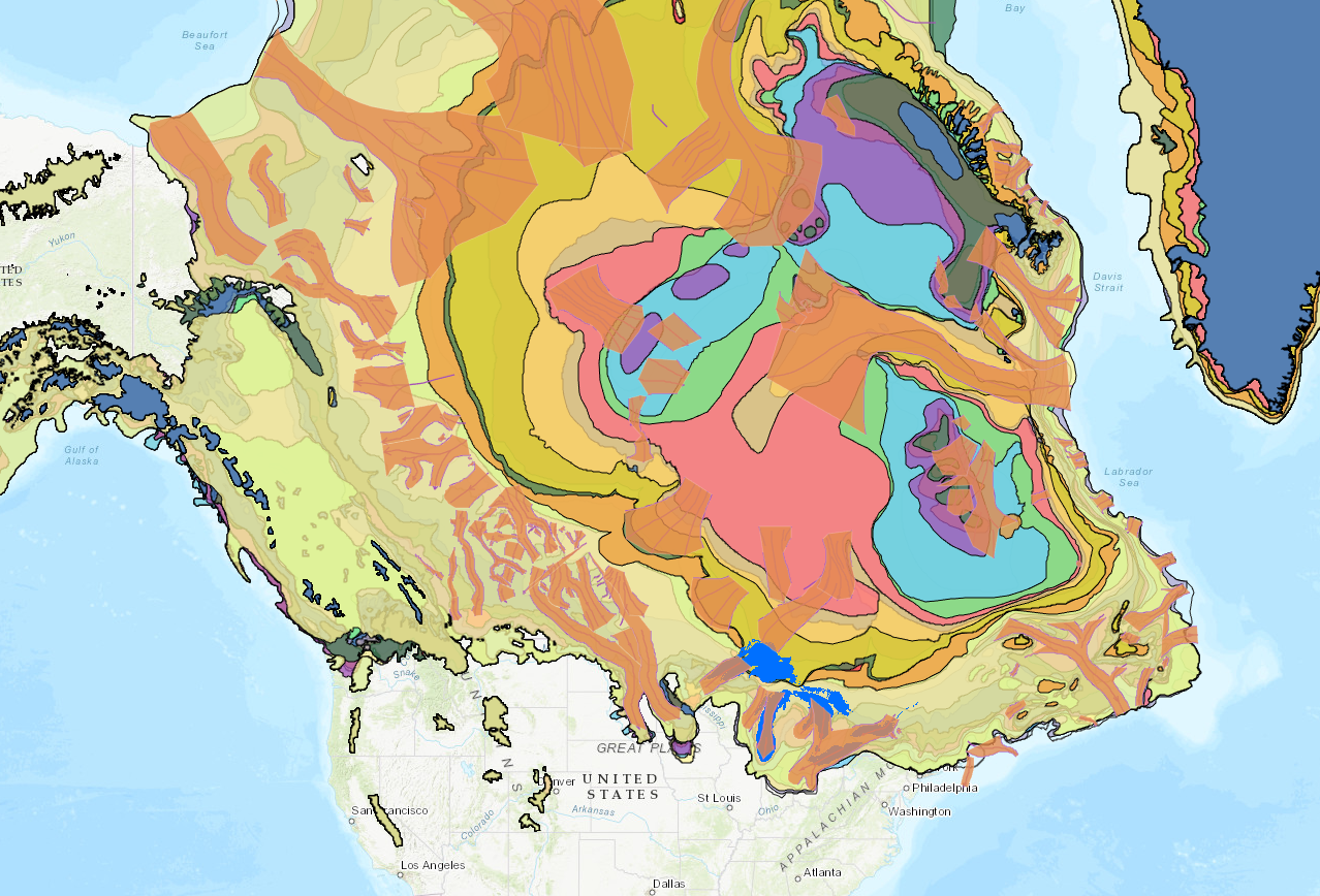
The Laurentide Ice Sheet during various glacial stages
The Laurentide Ice Sheet was a huge ice sheet, up to 2 miles in height in some places, with cycles of growth and retreat several times over the Quaternary period, from over 2mya to… today!
The geology of Minnesota is varied. There are alternating bands of igneous and sedimentary rocks. In the north, a range of mountains several kilometers high was created by tectonic compression, made of strong metamorphic gneiss. In the Arrowhead region in the northeast, located near to Lake Superior, tectonic tilting has exposed weaker, lesser-jointed shale rocks.
Its last advance occurred between around 100kya and 20kya, where subglacial erosion carved out areas of North America, from the huge Hudson Bay to the hundreds of thousands of smaller lakes present in Minnesota and Canada, such as Mille Lacs Lake in an ellipsoidal basin. The mountains were eroded; now Eagle Mountain, the highest, is only 701m high. Part of Lake Superior and other Arrowhead region lakes were deeply eroded thanks to their weaker geologies.
As it made its final retreat, meltwater was blocked by the ice and the large “Big Stone Moraine”, forming Glacial Lake Agassiz. It was larger than every Great Lake combined, covering around 300,000 square kilometres, around the same size as the present-day Black Sea. With continued ice ablation, a glacial lake outburst flood (GLOF) occurred as the moraine was overtopped, around 11,000 years ago, resulting in large-scale erosion of an area 8km wide and 76m deep in Browns Valley, Minnesota. This old river is known as the Glacial River ‘Warren’, helping to carve out the modern Minnesota and Mississippi rivers, and the valley present today. With the water came deposition: large swathes of fertile silt and soil deposits have been left behind in the valley, likely from the Big Stone Moraine. It took around 2,000 years for the lake to fully drain, and it likely had a large impact on the climate, sea level and even early civilisation! [simplified]

The top left is the bed of Lake Agassiz, and the eroded area is visible too. North Minnesota.
If you’re interested, an interactive map of the glacial extent and lobes is available here, thanks to the brilliant geographers over at Royal Holloway uni.
Ice Lobes
There are three phases of the glaciation period you need to know, with four associated lobes. Lobes themselves form because ice wants to move under gravity, and with the Laurentide ice sheet at 2 miles high, the base of the ice sheet was under significant pressure. The thickness of the ice above, topography of the land and geology have an impact on how lobes form. In areas of lower resistance such as a valley, ice can be channelled and advance faster, forming the lobes.
Wadena Lobe
The Wadena Lobe was the first of the four main lobes that were on top of Minnesota. Arriving around 30kya, the lobe came in from the north to north-west and is characterised by the deposits it created, being from red sandstone, shale and limestone.
This deposition produced the Alexandra and Itasca moraines, forming the tilly Wadena Drumlin Field over the Wadena, Otter Tail and Todd counties, and its ground moraine reached just south of the present-day Twin Cities.
Rainy and Superior Lobes
The Rainy Lobe moved in from the north to northeast of Minnesota and deposited the St Croix moraine, made of greyish, brown greenstone around 20kya.
The Superior lobe came in from the northeast at the same time. Partially covering present-day Lake Superior, it deposited a series of basalt, red sandstone and greenstone till moraines extending southwards to the Twin Cities. Like Wadena, it too deposited drumlins.
Des Moines lobe
The Des Moines Lobe was active during the most recent glacial period (LGP), around 13kya. It moved in from the northwest, covering vast expanses of the west of the county from the most northerly point to the most southerly point. It deposited till that is tan to buff coloured and is clay-rich and calcareous due to its shale and limestone source in the northeast. In the southwest, the Prairie Coteau region has examples of terminal moraine, and outwash plains. Many of this lobe’s deposits are over 160 metres deep in the region.
Post-glacial modification
Isostatic readjustment occurs when these ice sheet glaciers retreat due to the land not being under pressure anymore. This land then typically rebounds upwards and elevations increase in the area where glaciers once lay. Fluvial activities continued to mould the landscape after full glacial retreat had occurred.
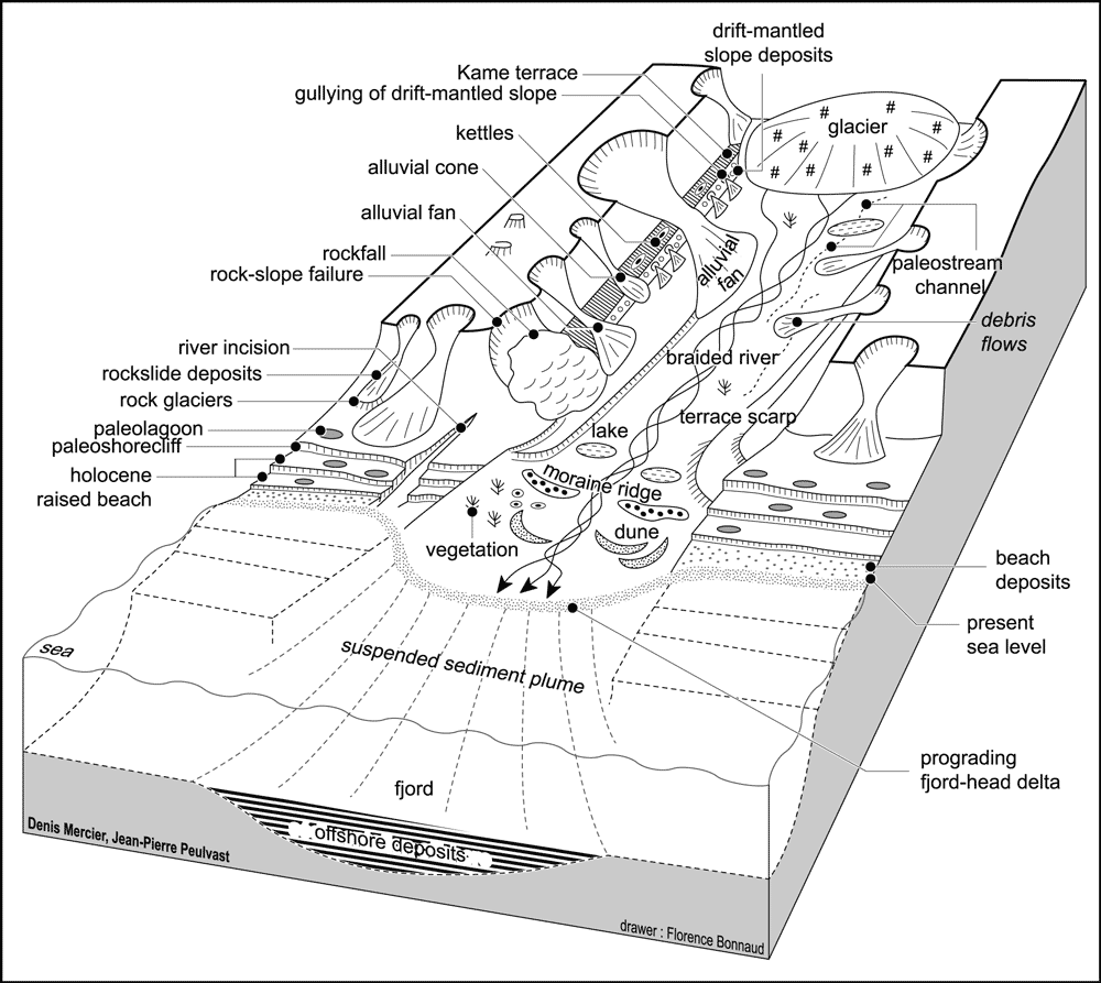
Glacio-fluvial landforms
(Date studied: 23/11/2022)
Glacio-fluvial means an environment shaped by glacial meltwater.
Geomorphic means changes (morph) to the land (geo).
Glaciofluvial landforms are formed as a result of climate changes during and after glacial periods.
Eskers
Eskers are long, sinuous (many curves and turns) ridges made from sand, gravel and other types of glacial till deposited on valley floors by glacial meltwater flowing through subglacial and englacial tunnels.
Eskers are “elongated ridges of glaciofluvial sediment deposited by subglacial meltwater pipes”.
These tunnels and channels over time become filled up with sediment. During deglaciation, this sediment is dropped onto the bedrock leaving stratified ridges, signifying that a glacial meltwater tunnel was somewhere above it. This could be either a kame (see below) or an esker.
The general consensus is that the deposition is caused when pressure is released at the glacier’s snout, so as the glacier retreats, the point of deposition retreats too. This can describe their beaded appearance (vary in height and width throughout) with the beads of greater size representing periods of relatively slow retreat, or halted ablation. Others may say that the larger beads are caused as a result of the greater load carried by the meltwater in the summer seasons.
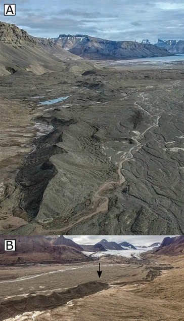
Here are 2 angles showing what they look like, in Svalbard.
The weight of the ice above the subglacial tunnels means that the water flowing within these subglacial tunnels is under extremely high pressure. When the ice melts, this pressure is released, so therefore dropping sediment.
Eskers are deposited unaffected by/ignorant of local topography, meaning that they can traverse over hills in the landscape.
The path taken by this pressurised meltwater is mostly controlled by the slope, size and direction of the ice surface rather than the bedrock. Because of this, eskers can be used to show the slope of the ice surface, as well as its extent! It also runs parallel to the direction of ice flow, running transverse to the glacial snout.
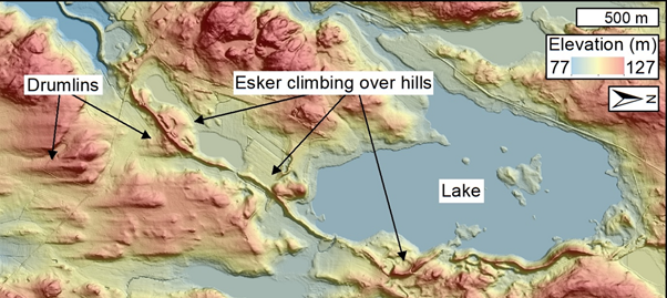
Topographic view of depositional landforms.
Eskers on paleo-ice-sheet beds are more abundant in areas of crystalline bedrock with thin coverings of surficial sediment than in areas of thick deformable sediment, because meltwater flowing at the bed is more likely to incise upwards into the ice to form an R-channel where the bed is hard; where the bed is deformable, meltwater is more likely to incise downwards.
You don’t need to remember that.
Examples
Many eskers are found in central Ireland, some are in Canada, as well as many in Iceland and Sweden.
Here is an example of an esker on Google Maps.
A meltwater stream is visible south of it, as well as another esker to the east.
Post-glacial climate change in Eskers
During periods of increasing global climatic temperatures, the rate of glacial ablation increases and results in more meltwater being produced. This means that there is more accumulation of sediment in proglacial areas and the length of these eskers is likely to increase or become more beaded with greater and more intense ablation periods. With faster glacial ablation, eskers will be exposed in greater number.
Kames and Kame Terraces
A kame is an irregularly shaped hill, hummock or mound made of stratified glacial till comprised of mainly sand and gravel.
There are two types of kame:
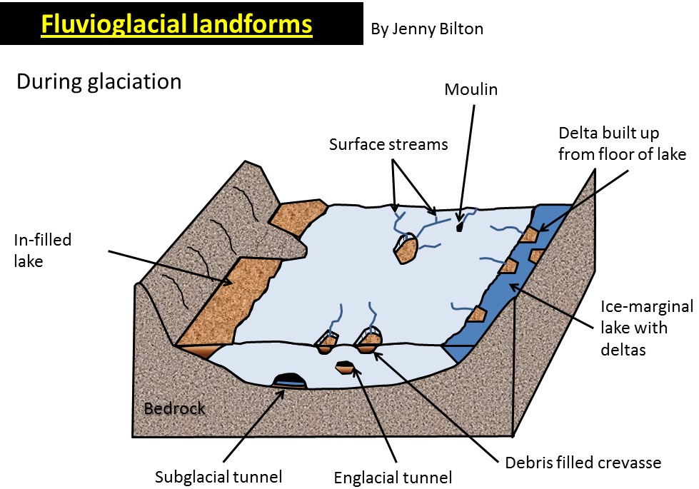
Delta kames
Delta kames can form in two main ways. Firstly, they can form due to the build-up of debris in englacial tunnels (and crevasses) that emerge at the glacial terminus as a result of retreat. As a result, they lose their energy, and are forced to deposit their contained load.
Another way that they can be formed is when supraglacial streams meet ice-marginal lakes. These ice margin water bodies are largely static (just sit there tbh) so the sediment they carry loses energy and gets deposited in the lake, from where this supraglacial stream enters it, often leading to a tall accumulation.
Kame terraces
Kame terraces are ridges of material near or on the valley margin. They are largely comprised of ex-lateral moraine, which was transported into the ice-marginal lake due to the supraglacial streams formed due to the warming of ice through friction with valley walls. As this is largely glacio-fluvial, unlike morainic deposits, these are somewhat sorted and stratified by the movement of water. When the glacier retreats, this sediment is dropped and collapses onto the bedrock floor.
Watch out! Many people say ‘kame’ when they mean ‘esker’! You need to know the differences between the two well. (main one is eskers are subglacial, kames are not)
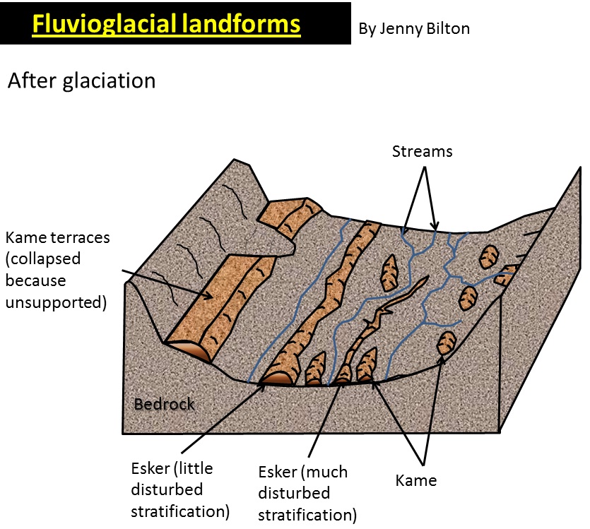
This displays the distinction between kame and esker.
As climate change increases temperature levels, more meltwater is present, which transports and deposits sediment. This will result in a larger amount of all types of kame being more likely to form.
Here is an example of an esker on Google Maps: https://www.google.com/maps/cheatsheet-esker-link
A meltwater stream is visible south of it, as well as another esker to the east.
Essay example: Explain the influence of climate changes and geomorphic processes in the formation of glacio-fluvial landforms
Kames are mounds of sediment deposited by glacial meltwater or ice, found in areas where glacial ice melted and receded, leaving behind sediment deposits. The process of kame formation is complex and is a result of a variety of interrelated factors, including climate change and geomorphic processes.
Climate change is one of the most significant influences on the formation of kames. During the Pleistocene epoch, large areas of the northern hemisphere were covered in thick glaciers. As the climate warmed and the glaciers receded, large volumes of meltwater were released, carrying sediment with it. The sediment was deposited in stratified piles, forming these kames, visible in places in the UK such as the Scottish Highlands or the Lake District. This can be proven to be the result of a glacio-fluvial deposition as they are deposited in one go by melting ice, while previous meltwater surface streams moved the sediment into crevasses or glacial marginal lakes.
Geomorphic processes also play a role in the formation of kames. As the glacier erodes the landscape, valley sides’ sediment may fall onto the glacier, ranging from large boulders to sand grains. The size and shape of these kames vary depending on the type of sediment deposited, as well as the rate of erosion. In addition to erosion, other geomorphic processes can play a role in the formation of kames such as weathering. These processes such as frost-shattering and chemical weathering can break down sediment particles and form smaller particles that can be easily carried by wind or water. This can cause further accumulation of sediment in certain areas and contribute to the formation of kames. Lithification may also occur when the sediment is compacted and cemented together, forming a solid mass among the trapped sediment.
In conclusion, climate change and geomorphic processes are both important factors in the formation of kames. Climate change causes the glaciers to melt, releasing large volumes of sediment, which is then deposited in strata. Geomorphic processes, such as erosion, sedimentation, and lithification, also contribute to the formation of kames. Together, these two factors contribute significantly to the formation of kames, alongside many other factors like the topography, aspect and relief of the local region.
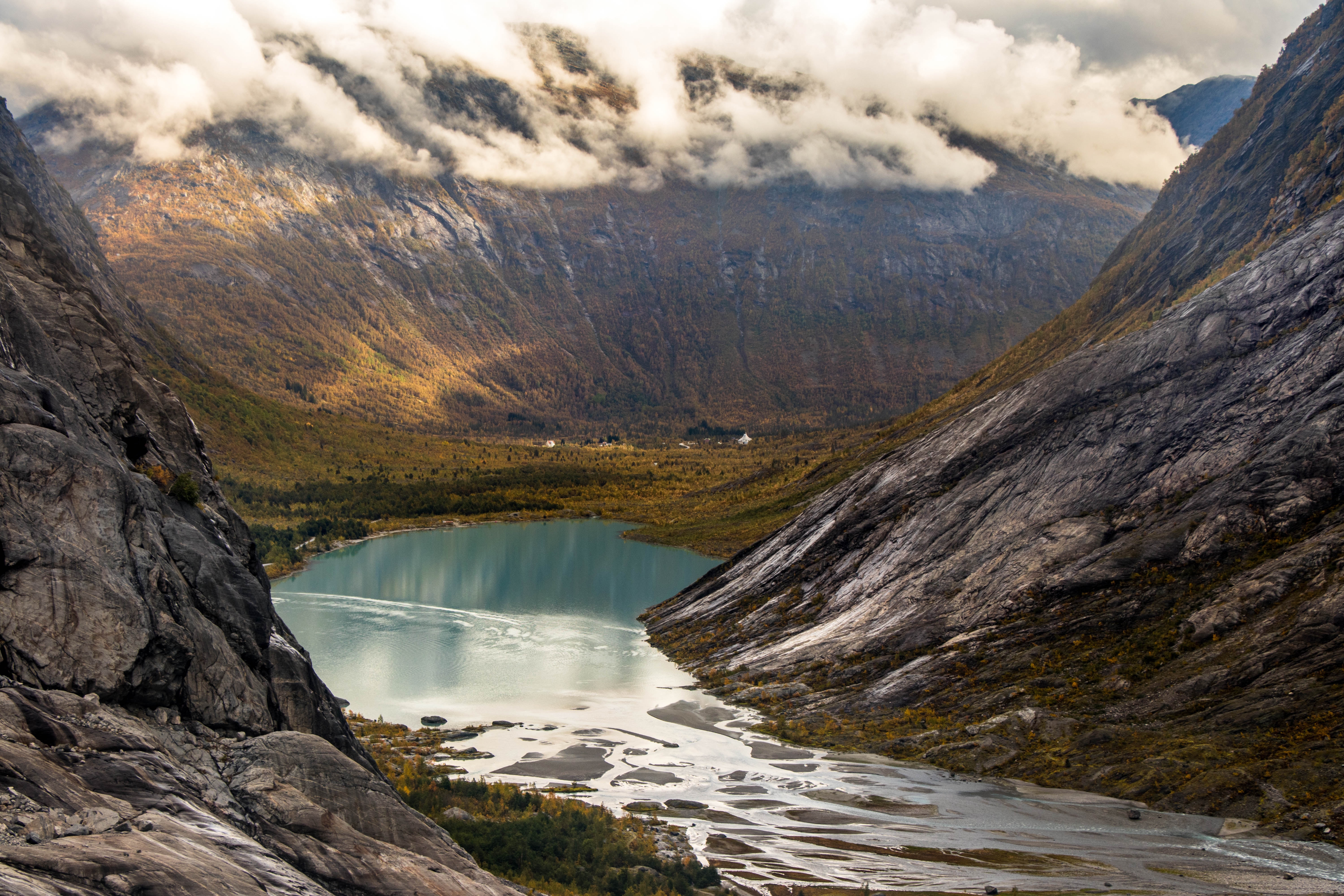
Proglacial lakes
Proglacial lakes form in front of glaciers, usually when meltwater streams become blocked by terminal moraines, glacial dams (trapped against a large ice sheet) or due to isostatic depression of the lithosphere into the weaker asthenosphere.
The meltwater, over time, accumulates in this area, unable to flow outwards. This is similar to how a traditional valley glacier system starts with the corrie melting and a tarn being left due to a terminal moraine blockage.
After a glaciation period, the climate typically warms up. Over time, if there is a large ice sheet blocking the water flow, this sheet will ablate, and the lake will either overflow or undermine the dam, causing a glacial lake outburst flood, or jökulhlaup.
Modern example: The Russell Fjord in Alaska is regularly blocked by the Hubbard Glacier, which can increase water levels in the fjord by up to 15m as it cannot empty out into Disenchantment Bay: Google Maps/3D Google Earth.
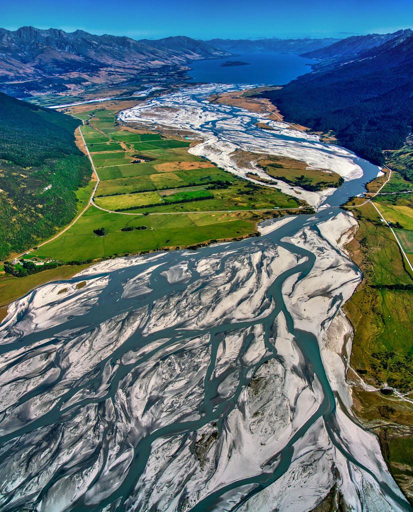
Outwash plains
Outwash plains are also known as sandurs. They are dominated by other landforms, including braided streams and kettles. They occur in front of melting glaciers, and are mostly flat and expansive areas. Meltwater traversing this terrain has little energy, and therefore little vertical erosional power and is more inclined to deposit material. As a result, these flat areas are created from stratified (strata; layered) sediment.
As the glacier moves over bedrock, plucking and abrasion (erosion) occurs resulting in silt and sediment being carried in this meltwater. Braided streams are dominant in outwash plains. These are very shallow streams and rivulets which carry and redeposit till due to the little energy in the system.
In summer months, there is typically higher glacial discharge and ablation, resulting in these tilly islets being destroyed by water, which has a little more energy due to increased velocity. This leads to more erosion, and these islets then go on to reform later. This makes the outwash plain have a distinct look. This can be described as dynamic.
The elevated level of erosion is typically closer to the glacial snout but then progressively loses energy.
In areas that were once glaciated, old outwash pains can be found by looking for sediment, with large angular rocks and boulders being present closer to the glacial mass and smaller, smoother rocks and sediment being further away from the glacier, similar to a typical river system aside from their origin. Outwash plains can extend for miles beyond the glacial margin (terminal moraine).
Braided streams
The general consensus is that braided rivers form instead of meandering rivers due to a higher sediment load, caused by discharge from ablation, as well as variable rates of flow.
At the end of a melting period, these lose water, lowering kinetic energy present in the system and therefore losing erosional power and increasing depositional power.
This results in material being deposited into the river channel, causing it to divide in two. Braiding itself develops when this ‘mid-channel bar’ grows downstream, as a result of more, finer material being added to the bar as discharge amounts continue to decrease. These bars, during times of exceptionally low discharge like in winter months, may become home to vegetation, becoming even more permanent. whereas unvegetated bars are less stable and often move with high discharge.
Many of these channels branch from other channels and merge to give it the ‘braided’ pattern. They are common in outwash plains due to the variable nature of ablation and meltwater amounts.
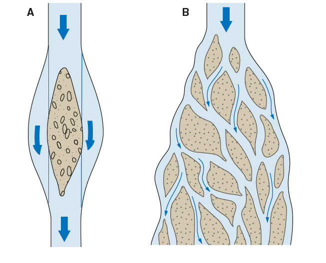
diagram of a braided stream
They are found in large quantities in south Iceland, for example.
Due to climate change, braided streams may dry up due to smaller amounts of ice present in these areas, after an initial increase in ablation due to temperature rise. This initial increased sediment load will progressively decrease as the ice mass decreases.
As a result, there can be expected to be more eroded streams, being deeper and wider, inside this outwash plain, followed then by the area becoming dry and tundra-like. Whilst vegetation thrives in outwash plains due to the rich minerals present in the glacial meltwater, this may also dry up in the future, becoming a barren, sandy and gravelly area with little life, or could be taken over and reclaimed by plants depending on resource availability.
Is that a braided stream AND a proglacial lake inside a valley glacier system?
Photo from Jonas Mendes.
Kettles
A kettle is a large depression in the ground formed by glacial deposition and is therefore a depositional landform. They create ‘dimples’ in the landscape around mountainous areas.
They are formed by large blocks of ice breaking from the main glacier. As the main glacier retreats, this ‘dead’ ice becomes stranded and, over time, becomes buried by sediment deposits as meltwater flows around it from the main glacier. Of course, this ice melts and its water evaporates, leaving behind a large depression, or kettle holes. Water can then fill these in again, or if not all water drains originally, resulting in kettle lakes.
Periglacial landforms
Periglacial landforms exist as a result of climate changes before and/or after glacial periods.
Periglaciation is concerned with the process and landforms attributed to the action of freeze-thaw, typically in permafrost areas.
Being in a periglacial area means an area that is near to, or on the fringe of, glacial areas’ ice mass, such that permafrost is present. This means that there is no physical glacier system present in the area, but it is still cold, relative to surrounding environments.
Permafrost
This is also part of the Earth’s cryosphere, as well as glaciers, ice sheets, and more!
Permafrost itself is comprised of:
- the active layer (this is the top few metres or so. It is warmer as it is closer to the surface. It may become unfrozen during the summer months and vegetation may grow too.)
- the permafrost layer itself.
- talik (year-round sections of unfrozen ground, soil, and rocks that lie in permafrost areas, but itself is not frozen)
There are 3 types of permafrost:
- Continuous permafrost: there is little thawing, even in the summer. These are often in areas of high altitude and latitude.
- Discontinuous permafrost: There are some patches of consistent permafrost, but are broken up by talik extending to the active layer
- Sporadic permafrost: small amounts of permafrost largely enclosed by talik
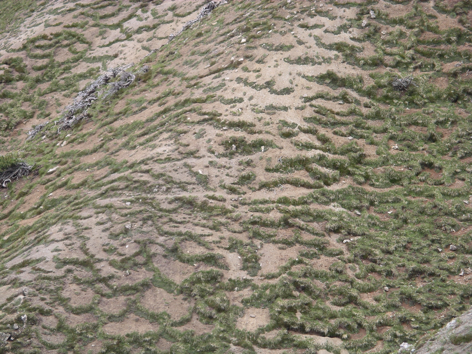
Patterned ground
This encapsulates sorted stone polygons, stone stripes, etc.
These landforms are facilitated by the process of frost heave. Stones within the ground and active layer have a lower specific heat capacity, allowing them to cool down and heat up faster than their surrounding soil. Due to the freezing conditions, water below the stones freezes as well, and also expanding by 9%, pushing the stones upwards. Over time and many years potentially, the stones are pushed to the surface, and to a larger extent, the frost heave sorts all fine and larger material too, creating a domed surface! How exciting.
Stones which are on top of this dome then fall down to undomed areas because of gravity. This is typically every 1 to 3 metres. These rows of stones can end up connecting and forming polygonal shapes.
On slopes, between 3 and 50 degrees, these polygons become warped and are known as elongated stone polygons, or garlands. On even steeper terrain these become stone stripes.
Blockfields
Lord help me if this comes up in the exam (I am not religious)
Blockfields are believed to be formed as a result of chemical and mechanical weathering below the active layer in periglacial regions such as plateaus or mountain tops, as these are typically glacial fringe regions rather than ice-covered areas.
Over time, these processes produce an uneven, angular & bouldery landscape which is only revealed after the permafrost layer melts away, forming ‘in situ’ (alternatively by rock glaciers - which are glaciers containing a large amount of frost-shattered rocks.). Blockfields potentially formed 23 million years ago during the Neogene epoch, when the climate was relatively warmer than today; higher amounts of chemical weathering then initiated the (very slow) process of eroding formed bedrock.
Resistant rock, or tor, may be more prominent in these blockfields as they are not as susceptible to denudation (erosional processes).
On slopes above a gradient of 25o, block streams/stripes are formed as gravitational forces will move this material down a slope.
Types of mass movement
Solifluction lobes
Solifluction refers the movement and “flowing” of soil and sediments.
When the ground and soil on slopes is frozen during the winter, the soil particles are separated slightly and loosened by the ice which forms and expands by around 9% between these particles (frost heaving).
During the thawing of the active layer in the spring and summer months, water saturates the ground as it cannot drain easily (due to the impermeable, frozen permafrost below - it is forced to stay in the upper layer) or evaporate due to the cooler climate. Friction is reduced between these particles, which are already loose after the freezing months, as this water can lubricate them. As a result of this excessive lubrication, the soil moves downslope easily. (The extra mass from the water can also help with this.)
Soil/Frost Creep or Mass Wasting
This is a process which moves material down a slope by a few centimetres per year even on high gradients.
When the soil freezes, the particles within the slope are lifted vertically at a 90-degree angle to the slope. As the soil thaws and the particles settle, they end up slightly lower than their original position. This process is repeated over time, gradually causing the slope to shift downward.
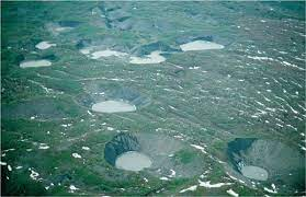
Pingos
Pingos are ice-cored hills in periglacial areas. Whilst they look the same and can be easily identified, there are two ways in which they form. They take several hundred years to form and only grow by a few cm/year. Large pingos visible in Canada and Greenland may be 600m wide and 50m tall.
During warmer climatic periods, the ice lens can melt, collapsing the dome of land above and leave a depression, typically a marshy area called an ognip, which is surrounded by “ramparts” of soil. Collapsed pingos in Wales are evidence for prior glacials and may only be 10m in diameter.
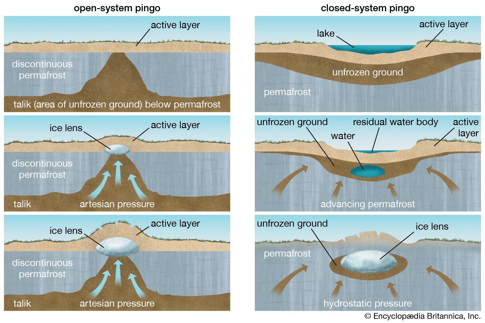
Open system, hydraulic
These are also known as East Greenland-type pingos as they commonly occur there.
Open system pingos form in areas of discontinuous permafrost, such as floors of valleys. Groundwater moves through the permeable talik and, through artesian pressure, moves upwards and cools. It feeds the ice core between the active layer and permafrost above, resulting in the ice core growing in size. Over time, the active layer above is pushed up, creating a dome of land visible on the surface.
Closed system, hydrostatic
These are also known as MacKensie-type pingos.
Closed system pingos are formed in areas of continuous permafrost. They develop in flat areas below lakes. The talik (typically fine soil, sediment or sand) below the lake is saturated by the lake, and remains as talik due to the lake’s relative warmth. Over time, the lake may become infilled with organic matter or sediment (or the water drains), reducing its insulating effect.
The permafrost thus is able to advance, surrounding the area of saturated soil, even trapping it by advancing between the saturated area and lake. Gradually the permafrost continues to advance, putting the water under hydrostatic pressure and making it rise upwards where it meets the cooler permafrost. This forms the ice core, and the hydrostatic pressure continuously feeds the ice, pushing the land above upwards into the familar pingo shape.
Ice-wedge polygons
Soil cracks when cooled quickly, just like how mud cracks when dried.
In summer, this crack in the soil fills with meltwater. Over time as many freeze-thaw cycles occur, the ice is expanded by 9% each time. This eventually results in the formation of an ice wedge. Each time the water is refrozen into ice, pressure against the surrounding soil increases, causing it to be pushed upwards, contributing to the development of these polygonal features.
Summary: Soil cracks when cooled quickly. In summer the crack fills with meltwater, and as it refreezes many freeze-thaw events take place, expanding the ice by 9% each time. This eventually results in the formation of an ice wedge.
Human activities in Glacial and Periglacial Landscape Systems
4.a. Human activity causes change within periglacial landscape systems.
4.b. Human activity causes change within glaciated landscape systems.
Case study: Oil extraction in Alaska (Periglacial)
Part of Alaska is located within the Arctic Circle, at 66.5oN.
However, since 1968, vast amounts of oil reserves have been found offshore and within Alaska itself, including inside the ANWR (Arctic National Wildlife Refuge) and, more specifically, Area 1002 within it. An estimated 12 billion barrels of oil is located in this area alone, with half of it (~6bn) being available to extract using currently available techniques.
For the United States, this would provide a key resource for energy security, while at the same time reducing dependence on foreign, potentially malicious, entities, which may limit their supply, such as Russia. This weakness has been seen in Europe, with Russia’s invasion of Ukraine, so now more than ever the US sees this as essential.
It imported 37% of its total oil consumption in 2016 (7,259,000 barrels per day).
Hydrological processes
Gravel extraction adds insult to injury. The loss of gravel from fluvial systems can change the composition of the river profile and exacerbate damages further downstream from the extraction site. Extracting gravel from a glacial outwash site has been proven to lower the groundwater levels by over a metre in a 2km radius as well.
Urban heat island effect
Barrow, Alaska is the northernmost settlement in the USA and the largest native community in the Arctic, with a population of 4600 in 2000, increasing from just 300 in 1900. Recent decades have seen an increase in mean annual and winter air temperature, with an earlier snowmelt in the village and a weaker snowmelt trend in the surrounding tundra.
The urban heat island (UHI) effect is a phenomenon where urban areas are significantly warmer than their rural surroundings due to activities by humans, like air conditioning, hot water pipes and road building.
A strong urban heat island (UHI) was found during winter, with the urban area averaging 2.2 °C warmer than the hinterland. There was a strong positive correlation between monthly UHI magnitude and natural gas production/use, ultimately resulting in a 9% reduction in accumulated freezing degree days in the urban area.
This excess heat is mostly generated from:
- The burning of fossil fuels during flaring. This increases the carbon dioxide concentration in the local atmosphere, resulting in an enhanced greenhouse effect. This increases the amount of terrestrial radiation within these areas.
- The absorption of solar radiation by urban surfaces - solar insulation warms up these more than surroundings as tarmac/gravel structures are black, which absorb more radiation.
- The reduced evaporative cooling from vegetation.
As a result of this input imbalance, permafrost can thaw, leading to changes in the landscape and the release of trapped carbon dioxide and methane, which can further contribute to climatic changes in these areas locally, as well as internationally, as permafrost contains 1.5 trillion metric tons of carbon (that’s 1,500 petagrams if you’re fancy like that - or double than what’s in the atmosphere today).
This thawing can furthermore lead to infrastructure damage, as roads and buildings can be damaged by the shifting of the ground due to solifluction.
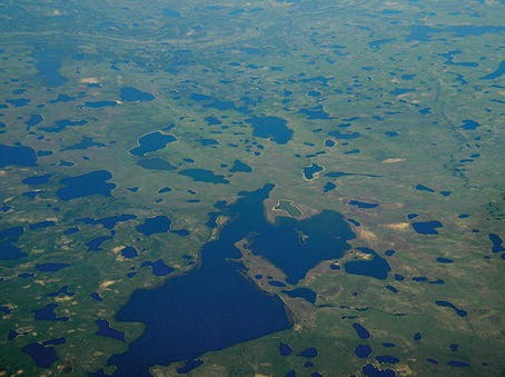
Thermokarst
A landscape characterised by depressions due to the thawing of the ground ice which comprises the active layer and permafrost below. Visible in the Alaskan North Slope.
Case study: Kárahnúkar HEP Dam, Iceland
This dam (or, collection of three dams) was built in East Iceland on a large proglacial lake, sourced from one of the largest glaciers in Europe. It is actively retreating, so provides water to the dam which can then be used as hydroelectricity. The dam itself was finished in 2007 and is large enough to be seen from space.
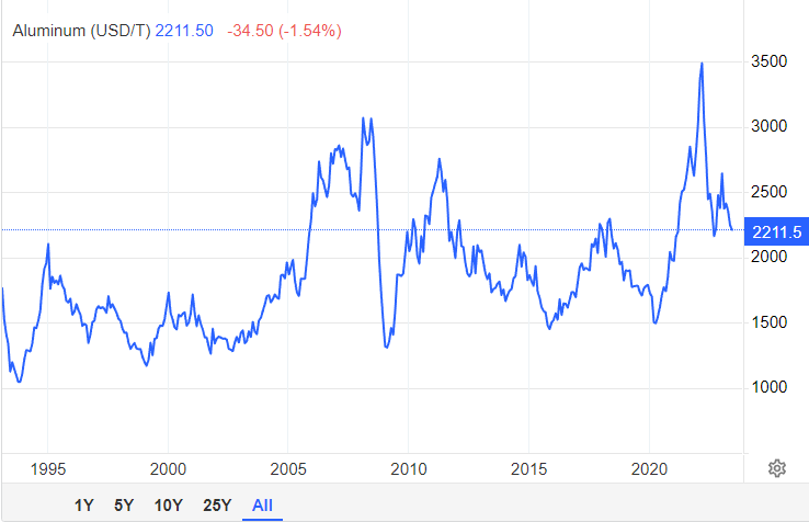
The dam could provide enough energy for all Icelandic homes and small businesses, but instead, all energy provides the nearby aluminium smelter called Alcoa.
However, there has been widespread backlash over the project, as it flooded over 400,000 acres of unspoilt highland wilderness which was the second largest unspoiled area in Europe. In total, almost 750,000 acres of land was affected by the construction of the dam, which is around 3% of Iceland’s total land mass.
The dam was built as Alcoa produces 2% of the world’s aluminium supply, and global financial markets at the time of construction were expected to make a significant number of jobs, and this aluminium industry was expected to make up 10% of Iceland’s total GDP. This has not happened yet, and the price of aluminium had almost halved just two years after construction finished, and has not recovered to this level seldom for market bubbles seen with the Russian invasion, which stressed productions of almost all raw materials.
Glacial meltwater, or glacial milk, is released by the Vatnajökull glacier and flows into the lake blocked by the dam. This glacial meltwater is known to have a high concentration of sediment within it, and as such reduces the capacity of the dam over time. This is because the suspended sediment at the base of the water solidifies when deposited, as there is little kinetic energy at the bottom to keep suspended sediment floating. Over time, the base level of the lake increases, reducing overall water capacity, until this excess sediment is ‘purged’ by the dam management system, which may happen annually.
Here’s a video of sediment getting purged, and here’s another one!
That’s the end for glaciation! I hope you found it useful.
What if I told you about Paraglaciation and Paraperiglaciation as well?
Earth’s Life Support Systems
“Without water and carbon I literally would not be here” - a wise man, 2024

giving earth life support - created with dall-e 3
1. How important are water and carbon to life on Earth?
The short answer to this is that the water and carbon cycles are very important.
The long answer? Well…:
Introduction to water
1a. Water and carbon support life on Earth and move between the land, oceans and atmosphere.
Water is a fundamental prerequisite for life, not just on Earth but it is considered by scientists as an essential necessity for any sort of life in the universe.
The Circumstellar Habitable Zone, or Goldilocks zone, is the habitable area around a star that is neither too close nor too far so that conditions for life are too hot or too cold, and categorised by allowing liquid water to be present. Otherwise, the water would be evaporated or be as solid ice. As such, liquid water allows life to form. Depending on the star, this zone can be further or closer to it, or the zone itself being wider or smaller.
It is described by astronomers as:
“The area around a stellar object which contains liquid water, making it habitable. The regulation of temperature and radiation facilitate respiration and photosynthesis”.
Water is essential to supporting life. The atmosphere is sustained by a continual cycle of evaporation and condensation through cloud formation. Water vapour itself is a very potent greenhouse gas, which regulates and moderates global temperatures: the climate is 15 degrees C warmer with water than without. As sun rays collide with the molecules in water vapour, they heat them up, causing them to vibrate and let off heat. In addition, water vapour is excellent as stopping short-wave radiation from causing harm for the biosphere. The greenhouse effect by water vapour prevents some long-wave radiation reflected from the Earth from exiting. It makes up 65-95% of all the biospheric mass, including in people, flora and fauna.
Water itself is in a closed system, meaning that water cannot enter or leave the Earth. As the water cannot exit or enter, it is transferred, stored and moved around inside the system. This is known as the global hydrological cycle. An open system within the overall closed water cycle system may be a drainage basin: water can enter and exit at any time.
| Store | Size | % of total |
|---|---|---|
| Ocean | 1.33b km3 | 96.5% |
| Cryosphere | 24m km3 | 1.76% |
| Aquifers | 23m km3 | 1.69% |
| Lakes | 176k km3 | 0.013% |
| Pedosphere | 17k km3 | 0.0012% |
| Atmosphere | 13k km3 | 0.00093% |
| Rivers | 2.1k km3 | 0.00015% |
| Biosphere | 1.1k km3 | 0.000081% |
* Data updated to match latest scientific research.
Introduction to carbon

Carbon is the building block of life on Earth. It is available for use in the natural world and by humans.
It is found across the planet, in a wide variety of stores, and is measured in petagrams of carbon - PgC - which is the same 1 gigaton. It is stored as a gas in the atmosphere, in oceanic sediments, and is used in living organisms to… continue living, amongst other things. Carbon is also very useful as we can use it to power various electricity generators through hydrocarbons like oil.
Similarly to water, carbon is a closed system on Earth, but on a more local scale such as a rainforest it becomes an open system.
| Store | Amount | Format |
|---|---|---|
| Lithosphere | 100,000+ PgC | Fossil fuels, sedimentary rocks |
| Hydrosphere (deep) | 40,000 PgC | Mostly CaCO3 from dead shelled organisms and bicarbonate ions. |
| Pedosphere | 2,000 PgC | Litter from dead or decaying matter and near-surface soils |
| Cryosphere | 1,700 PgC | Permafrost |
| Hydrosphere (upper) | 1,000 PgC | Dissolved CO2 from atmospheric dissolution |
| Biosphere | 650 PgC | Living organisms, flora and fauna. |
| Atmosphere | 800 PgC | Carbon dioxide |
The data is somewhat variable and differs between scientific research.
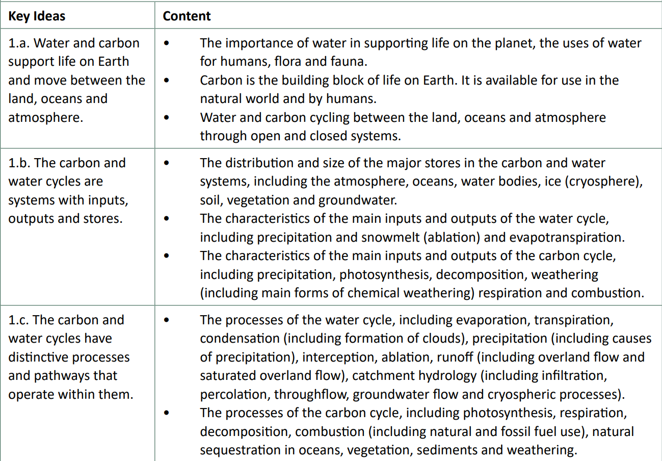
Inputs, outputs and processes of water
1b. The carbon and water cycles are systems with inputs, outputs and stores.
1c. The carbon and water cycles have distinctive processes and pathways that operate within them.
In the global hydrological cycle, there are many interrelated processes, stores, inputs and outputs, similar to that of a glaciated system. Flux is a term used to measure the rate of flow between stores, through mass over unit time (e.g. 3m/s). In total, around 505,000km2 of water is moved annually around this system.
Evapotranspiration
Evapotranspiration is the term used to denote the transfer of water into the atmosphere, combining evaporation and transpiration. Energy, such as insolation, when added to a mass of water like an ocean, increases particles’ energy and breaks the bonds between them, allowing for a state change to gas as water vapour, which then rises. This is evaporation. Transpiration on the other hand occurs only from the biosphere and mainly plants - this accompanies the process of respiration and photosynthesis. Leaves and plant surfaces lose water through their stomata via evaporation, and this water is replenished through effectively pulling more water and nutrients from the roots through the plant. On a local scale this may be insignificant but on a wider, perhaps national scale such as the Amazon Rainforest, the amount of water transpired through the plant, and evaporated by rivers and other stores, contribute significantly to changing global weather patterns. In total, transpiration accounts for around 10% of atmospheric water vapour.
Water in the soil (pedosphere) is the most likely to be absorbed by trees and vegetation, which transpire and release water into the atmosphere. You can use this as an example of a rapid flux, from the pedosphere, to the biosphere and then into the atmosphere, perhaps in under a day. An oak tree can transpire over 150,000 litres of water per year. In total 10% of water vapour present is transpired by plants (biosphere)!1
Precipitation
One of the main processes in the water cycle is precipitation. Simply put, this is when water leaves the atmosphere through any form, such as rain, snow, sleet or hail. When water vapour reaches the critical dew point (temperature at which air becomes saturated with moisture), it condenses in the atmosphere as clouds. Provided that there exists condensation nuclei, then clouds will form. As these nuclei of ice crystals or water droplets aggregate, they become too heavy to be suspended in the atmosphere, thus reaching a critical size and then fall to the surface as precipitation. This process is known as the collision-coalescence theory.
Water produced by precipitation is then collected in a drainage basin and moves into rivers through runoff - a combination of processes including overland flow, in addition to soil infiltration, ground percolation and subsequent throughflow and groundwater flow. Most of this water will then enter the ocean again, ready for the cycle to repeat, or percolate further into permeable rocks and be part of an underground aquifer.
Some key points:
- Where precipitation occurs at high altitudes or in cold environments, snow is likely to form, and potentially remain on the ground for a long time, increasing the lag time visible on flood hydrographs.
- Duration is the length of time a period of precipitation lasts. Climatic depressions or frontal weather systems may cause this; there may also be high rates of overland flow with flooding for long durations.
- Intensity is how much precipitation falls over a given time period. This can also have an impact on reducing lag times with high intensity, causing more overland flow due to less time to infiltrate into the soil. The amount the soil can absorb is the infiltration capacity.
- Precipitation may also vary seasonally, with greater intensity in certain months. This variation can increase or decrease the amount of water in rivers and lakes.
Precipitation may make it to the ground in a catchment area and be subject to the processes involved in catchment hydrology. Or, it may be intercepted by trees and vegetation,
Ablation
Ablation, which you might know from the Glaciated Landscapes unit, is the result of snowmelt. Glaciated environments and ice sheets contain the second highest amount of stored water on the planet - behind that of oceans - at 29 million cubic kilometres. Although most is in polar glaciers which take a longer time to melt due to the much colder temperatures, water is still released through meltwater, calving and sublimation. And from retreating alpine glaciers.
In addition, permafrost melting can also contribute to the creation of extra ponds and lakes, visible in thermokarst landscapes in the Arctic Tundra. This change occurs seasonally.
This video is a great example of the risks to humans when there is too much ablation. [VIDEO]
Condensation & cloud formation
There are some fundamental principles of cloud formation you need to know:
- HOT AIR CAN HOLD MORE MOISTURE THAN COLD AIR. (Greater energy allows for more gases)
- As air rises, it always cools, at a rate of 0.65 degrees C per 100m or so.
- Due to gravity, there are fewer molecules of air above the original air pocket. Therefore the pressure is lower, and the air pocket expands. With this expansion there is greater room for the molecules to collide, reducing kinetic energy. A reduction in energy lowers temperatures.
- Air rises when it moves over a mountainous region, or wind from below moves over a mountain.
- The atmosphere has less pressure with altitude. Therefore, the same amount of air in a ‘parcel’ will occupy a greater area at higher altitudes.
- The dew point is the critical temperature at which air can contain purely water vapour at a given pressure. Beyond this point, cooling results in condensation as no more moisture can be held as vapour.
Air moves in ‘parcels’ which have their own temperatures, humidity, etc.
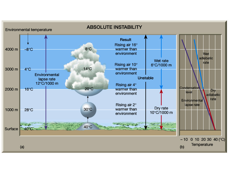
Adiabatic expansion
When air cools or expands adiabatically, this means that there is no heat exchange with the environment. The parcel of air purely changes based on the pressure being exerted on it by the atmosphere.
- The environmental lapse rate (ELR) is the decrease in air temperature with altitude for a specific time and place. this is 6.5 degrees C per km on average
- The dry adiabatic lapse rate (DALR) is the rate at which unsaturated air cools during ascent, or warms during descent. The DALR is 10 degrees C per km.
- The saturated adiabatic lapse rate (SALR) is the rate at which air at its dew point (and therefore condensing) cools as it rises. Condensation releases latent heat, making this lower than the DALR at around 7 degrees C per km.
These are significant as the determine how “stable” the atmosphere is.
When the sun warms an area of land, it creates heat, which warms up the air around it. As this air is unsaturated, it will decrease in temperature at the DALR. As it continues to increase in altitude, the temperature reaches the dew point, and the air becomes saturated.1
Cloud formation
Clouds main form through convection. As an area of ground warms, the local air “parcel” rises - this is atmospheric instability. For this example, let’s say that the dew point is 10degrees C lower than the temperature at the surface (as a result of insolation). Therefore, as the air has not reached its dew point, it moves upwards at the DALR, and reach the dew point at an altitude of 1km. Once it reaches this level, condensation will occur, forming a cloud. However, there is still convection occurring, as the air parcel is still warmer than the surrounding ELR. Eventually, the ELR and SALR will be in equilibrium at a given altitude, which marks the point of atmospheric stability and halt of cloud formation
Different areas at different times have different dew points. and rates of ELR
This may be hard to visualise as we cannot see individual clouds and water rising and falling. I like to resolve this by remembering that it’s not one cloud that forms: it’s a whole cloud system that can span 1000s of kilometres; the sun can cause this convection after heating whole continental areas of land.
If the dry environmental lapse rate is lower than the ELR, the air parcel that would typically rise is unable to do so as it is cooler than the surroundings and can only rise through force (e.g. topographic changes) as the atmospheric conditions here are stable.
Ways clouds form
Air can be cooled, aside from just moving vertically upwards, in several ways, and they create different types of clouds.
- Hot air rises through convection, cooling through adiabatic expansion, in areas of atmospheric instability. This forms large, puffy cumulus and cumulonimbus clouds - rain and thunderstorms common.
- Air can move laterally over a cooler area, as advection. This includes nimbostratus clouds. (Remember, as they move into a cooler area, condensation is more likely, with higher dew points)
- Air can be forced through wind over an area of high topography (mountains) through orographic lift, cooling more rapidly and thus reaching the dew point more quickly, forming clouds on the windward side of the mountain. This creates orographic rainfall on one side and a rain shadow on the other.
- When a warmer air mass mixes with a cooler one, the cooler one is heavier and will slide below the warm one. This is frontal lift. The hot air above is lifted by the cool air below, rapidly cooling it and, if this is enough to reach the dew point, the air becomes saturated and clouds form!
Catchment hydrology
There are a range of processes in a drainage basin that affect the water cycle.
When precipitation occurs in an area above freezing point, is is able to move rapidly as water as opposed to slowly as snow. When this water lands on soil, it has a few options, ultimately with the goal of moving into rivers through runoff - a combination of processes, as defined below:
Overland flow is the term used for the flow of water over the ground. It is the same as surface runoff. When on the surface, water may infiltrate into the soil - provided that the ground is not saturated. If the ground is saturated, typically defined by the water table being at the surface, then the water running off on the surface is known as saturated overland flow.
When this water has infiltrated into the soil, it can move through it laterally through throughflow. Gravity still acts on it, and therefore it may percolate into permeable ground rocks, or aquifers. Water in these rocks are stored as groundwater, and move through groundwater flow. It may then move into a store such as ocean or lake, where it remains for long periods of time. Eventually, evaporation moves it into the atmospheric store.
Inputs, outputs and processes of carbon
Precipitation
I’m not sure why the specification specifically states this, as this is mostly to do with the water cycle. However, rainwater and other forms of precipitation can combine with gaseous carbon (CO2) to form carbonic acid, which is able to break down some sedimentary rocks in situ, such as limestone. In addition, in oceans, calcium carbonate is a store of carbon in plankton and shelled organisms, and this may precipitate when the organisms die and lithify on the ocean floor. However, as carbon is acidic, too much of this can disturb marine life.
Photosynthesis
Photosynthesis is the process that transfers atmospheric carbon dioxide into the biosphere, accounting for 120 PgC per year. Plant stomata open and close and allow carbon to enter, combine with water, to create energy (glucose) for the plant, allowing it to grow and increase its transfer of carbon further. The respiration flux accounts for 118 PgC to be transferred back into the atmosphere from the biosphere store too. This is an example of the fast carbon cycle.
Decomposition
Decomposers such as fungi and microbes break down dead organic matter, and in the process releasing most of the stored carbon into the atmosphere as carbon dioxide, and some into the soil too. This process occurs very quickly in environments where there is a lot of energy usually given by heat along the equator in tropical rainforests and is slower in much colder locations like the tundra.
Weathering
Weathering includes physical, chemical and biological components, and refers to the in-situ breakdown of rock.
Physical weathering is the action of other factors such as water or biotic life mechanically breaking down rocks, for example roots cracking open rocks or freeze-thaw action.
Chemical weathering can also be significant, such as carbonation, which occurs when carbonic acid is produced (see above) which breaks down carbonates in rock strata, which then releases CO2 gas or dissolved in water streams. This contributes to how phytoplankton and other cretaceous aquatic organisms obtain their carbon - and accounts for 300 million tonnes annually.
A combination of physical weathering, which increases the surface area susceptible to chemical weathering, and chemical weathering itself
Combustion
Combustion is simply the process of burning organic material with oxygen, releasing carbon and other gases.
The biggest example of this (10 GtC/yr) is human activities, from fossil fuels for power stations. This moves carbon from the lithosphere to the atmosphere.
In natural environments too this is essential lightning creating fires, removing forest floor litter and allowing new growth when spaces of the forest canopy are opened. This moves carbon from the biosphere, and sometimes soils and peat too, to the atmosphere.
Volcanism (Hazards)
Not part of the Paper 1, but a synoptic link can be made to volcanoes and how they release carbon for Paper 3, Hazardous Earth. As tectonic activity moves carbon that has been lithified on the ocean floor as sediment into the Earth’s crust and mantle, where the matter is heated and turned into a gas. At a convergent boundary, the gases bubble up and release the stored carbon from the lithosphere into the atmosphere. This is extremely slow, known as the deep water cycle, over millions of years, but when it does occur, can be significant. This accounts for around 300 m tonnes per year (40x less than anthropomorphic emissions). Source
Oceanic sequestration
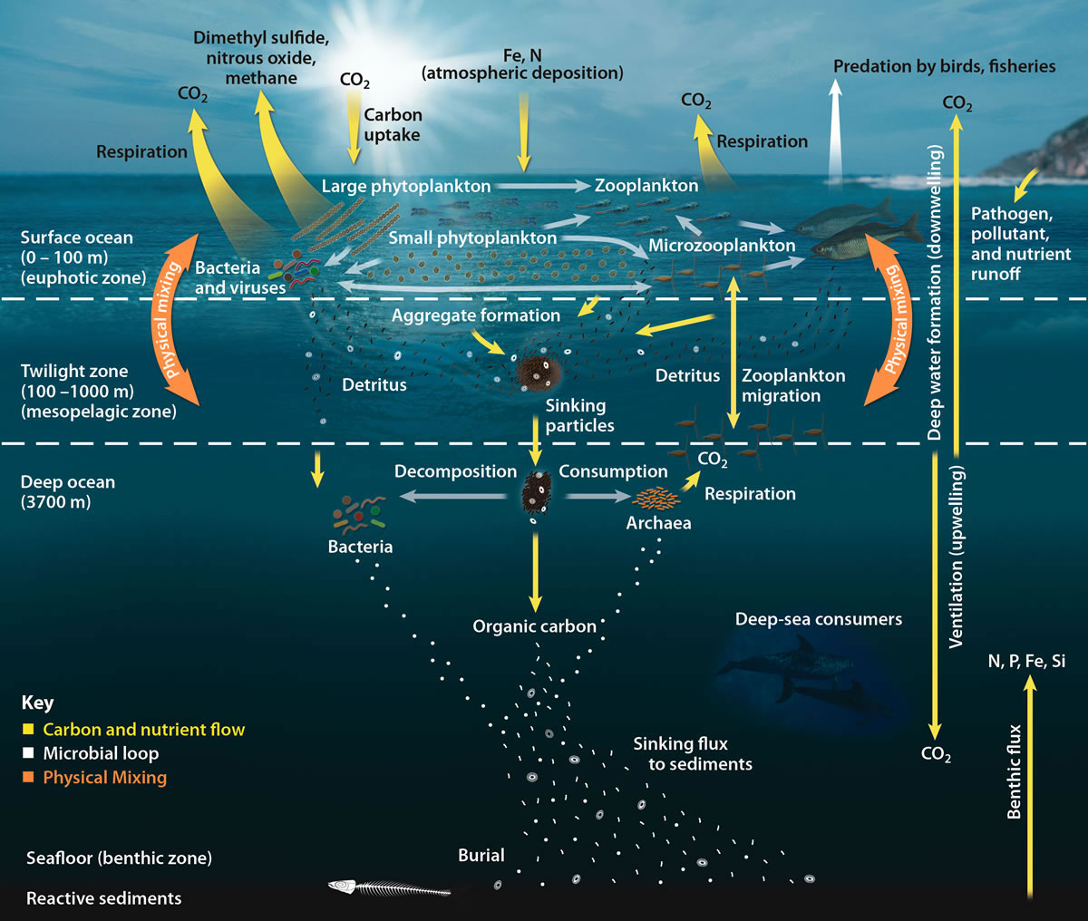
Oceans absorb large amounts of atmospheric CO2 through diffusion - there is a concentration gradient between the water and air. Currents move this carbon and the water too. In cool climates, water becomes denser, and it sinks - bringing the dissolved carbon within it too. This is an example of downwelling. As this is a cycle, upwelling may occur many thousands of years later in warmer climates.
In addition to this, phytoplankton and other marine life take in carbon from the atmosphere. This accounts for half of all photosynthesis worldwide, at over 50 GtC/yr! Phytoplankton are the basis for the marine food chain, with the locked carbon either falling into sediment on the ocean floor, or being eaten by other organisms like shelly crustaceans that then decompose (releasing CO2 gas) or, again, falling and eventually lithifying into sedimentary rock, being part of the long-term carbon cycle.
Vegetation
Vegetation, or the biosphere, takes in huge amounts of carbon and sequesters it for long periods of time. Rainforests, boreal forests and mangroves photosynthesise large quantities of carbon from the atmosphere. In general, for the first 100 years of a tree’s life, it is a carbon sink, and even after this period ends, the carbon sequestered is visible in its huge trunk and biomass store, potentially several tonnes of it. Some vegetation can store carbon for centuries.
Sediments
Sedimentary rocks include limestone, shale and sandstone. As sediment, from organic matter, builds up over time, the sediment at the base of an accumulation may be compressed and turned into rock, a process known as lithification. This process notably occurs at the ocean floor and accounts for 0.2GtC/yr from the hydrosphere -> lithosphere.
Case study: the Amazon Rainforest
2a. It is possible to identify the physical and human factors that affect the water and carbon cycles in a tropical rainforest.
You may have done this at GCSE - might be good looking back for a more general understanding!
Topical rainforests are almost exclusively located between the two tropics, at 23.5degN and S from the equator. They are categorised by:
- having high average temperatures (around 27degC)
- little variation in temperatures seasonally
- very high annual precipitation (>2000mm). Although the precipitation can vary seasonally, with Manaus recording 6x more rainfall in winter/spring compared to summer, there is no dry season.
- Net primary productivity (the net gain of carbon stored in an ecosystem) is about 2,500g/m3/yr.
Undisturbed tropical rainforests absorb over 30 tonnes of C/ha/yr, and respire 24.5t C/ha/yr. The amount of total carbon stored in all rainforests is around 100 GtC, with 1-3GtC annually absorbed from the atmosphere.
- There are ~390 billion trees in the Amazon. (around the same number of stars in our Milky Way galaxy)
70% of the Amazon is located in Brazil.
Physical factors affecting water
Water has many stores and flows in the rainforest. Water is affected by a variety of physical factors including:
- temperatures
- rock permeability and porosity
- relief
High temperatures allow the atmosphere to have high absolute and relative humidity, with a higher dew point. This allows large, cumulonimbus clouds to form with convectional rainfall from the heat, all year round. Diurnal changes in temperatures mean that precipitation occurs typically in the afternoons.
In addition, these high temperatures and the geographical location (between the tropics) mean that transpiration losses are high, but also the inputs into the plants are high, stimulating great plant growth, which in turn increase water uptake and evapotranspiration. Overall, 1/2 to 3/4 all precipitation is recycled (evaporated without any runoff), demonstrating strong interdependence between the land, biosphere and atmosphere with evapotranspiration and precipitation.
This is an example of a positive feedback loop: greater vegetation, greater evapotranspiration, greater precipitation, greater vegetation… etc.
Rock permeability in the Amazon is also a physical factor. The Amazon Basin is surrounded to the north and south by the Guiana and Brazil Shields, sections of ancient crystalline rock with high amounts of jointing, with the central Amazon River lying in between, in an area of weakness. This means that runoff rates are much higher for large portions of the Amazon, due to there being little potential to store and slow water movement during intense precipitation events, with short lag times. In the west, outcrops of limestone and other porous rocks can help to store water and reduce overland flows. In the long-term, huge water stores have built up in the underground aquifers and the soil, with a shallow water table of under 5m.
Relief also plays a role. The gentle relief of the basin today results in most flows being horizontal, either overland or throughflow in the soil. However, the Andes to the west increases the relief significantly. Higher relief adds energy to water and thus there is less chance for infiltration to occur. Surface runoff is much higher and, combined with orographic lift likely occurring here, there is the potential for low-lying flood plains downstream to fill for several months. Therefore, relief can both increase and decrease levels of overland flows, whilst altering the stores of water in the soil or over the land.
Physical factors affecting carbon
Carbon stores and flows are influenced by temperature, vegetation, organic matter in the soil, and rocks’ mineral composition.
Biomass, unexpectedly, is the greatest carbon store, with 100 billion tonnes of it. The temperature sustains strong rates of photosynthesis, which creates more plant matter and a positive feedback loop ensues, with NPP at 2500g/m3/yr. The amount of organic matter in the soil accounts for 40% of the rainforest’s total carbon store, showing there is significant storage and sequestration in the roots of trees. The growth is facilitated by high temperatures, which is strongly dependent on the interrelationship with the water cycle.
The high temperatures and demand for nutrients also make the store of carbon in and on soil very low, due to the very fast decomposition of dead matter by decomposers. Organic carbon thus circulates very rapidly.
The mineral composition of rocks, is largely igneous and metamorphic, with granite being abundant. These are not carboniferous but store large amounts of carbon in the long-term.
Spatial scales
An individual tree may have little influence on the cycle of water and carbon. Trees are the main factor in reducing the velocity of precipitation, shielding the soil and preventing runoff of nutrients. At the same time, detritivores and decomposers are sheltered from the sun under tree cover, allowing for rapid decomposition of nutrients and release of carbon on the forest floor. A single tree sequesters over 22kg of carbon every year from the atmosphere through photosynthesis fixation through the stomata of each leaf, permanently (well, until combustion or deforestation occurs).
An individual tree can take up around 50,000 litres of water every year from the soil. This is fuelled by uptake from the soil and groundwater stores, naturally reducing the amount of water there and adding it to the feedback loop of evapotranspiration and precipitation. They also play a part in intercepting precipitation, evapotranspiration and stabilising the soils through their roots, which are a large subterranean carbon store too.
The rainforest as a whole may create flying rivers due to the sheer amount of water being pumped by transpiration and the temperatures facilitating evapotranspiration. Huge amounts of water is transpired - 20 billion tonnes per day by the 390 billion trees acting as pumps from the soil to the atmosphere, so much so that there is more water in these flying rivers than there is in the Amazon River itself.
The Amazon rainforest stores over 100 billion tonnes of carbon and absorbs 2.4 billion tonnes annually, with 1.7 billion tonnes released through decomposition and respiration. This has a global scale impact, with it accounting for 1/4 of all terrestrial carbon absorption. Small changes in the carbon cycle thus have wide-ranging consequences.
Madeira drainage basin
This basin is located in the southeast of Amazonia and in Brazil, Peru and Bolivia. It accounts for about 20% of the Amazon’s area and is the largest tributary river. Deforestation has occurred in the higher elevation catchment areas, reducing the immediate storage of carbon and water in the biosphere and eroded soils. The outcrops of permeable rocks in this area, due to the velocity of water increasing and therefore less time for absorption, decreased in their water storage.
Downstream, flooding in 2014 caused the inundation of floodplains, and water levels at Porto Velho reached record levels at 19.68m above normal. There were 60 deaths, 68,000 evacuations and the longer-lasting effects of water-borne disease outbreaks including cholera. Unexpectedly high rainfall (exacerbated by orographic lift) combined with the reduction of interception, decreased lag times and increased the peak flow. Overland flows increased substantially, with water unable to infiltrate into the soil as much and percolate into aquifers, it was understandable that the overland flow in Porto Velho was too much, and the ground was full saturated by this point.
Impact of human activity
As already demonstrated, there is high interdependence between the land, biosphere and atmosphere. If just one of these are disturbed, there is a consequence on all the other aspects. According to REDD, between 10 and 20 per cent of global GHG emissions are caused by forest destruction and damage, which equates to more than the entire global transport sector!
70% of deforestation in the area is cattle ranching. In total, deforestation peaked at 20k km2/yr in around 2005.
The effects of deforestation are wide-ranging. Converting trees into pasture increases runoff by 27x. Rainforests also have significantly greater humidity and convectional rainfall versus pastures, decreasing the likelihood of cloud formation downwind from them. This can cause droughts and greater aridity at a national or global scale - studies have found that this moisture cycle regulates rainfall patterns in the western United States. Deforestation in one area makes other forests unexposed also more likely to be at risk through environmental degradation, potentially causing a snowballing effect of damages to not only the ecosystem but the carbon and water cycles at large.
On the carbon cycle, human activity shrinks the carbon stored in biomass by between 90 and 99% with grass or croplands versus the rainforest, from hundreds of tonnes per hectare to just two tonnes. Soils are depleted with less decomposer activity, and have nutrients, being washed away quickly with the precipitation not being slowed by throughfall or stem flow.
Deforestation also causes a degrading effect on other areas of land beyond the immediately deforested area. 38% of remaining Amazon forest already degraded - an area 10x the size of the UK and amounting to over 1 million km2; these areas exhibit similar (but somewhat less severe) characteristics to deforested regions.
All of these combined have resulted in severe droughts downstream for population centres in Rio and Sao Paulo. The lack of water in reservoirs and extreme heatwaves due to the South American climatic system no longer being in equilibrium as a result of human activity is stressing aquifers and groundwater stores further, which is unsustainable.
Management strategies
Several management strategies that preserve and have positive effects on the water and carbon cycles are in use today.
Legislature
Almost half of the Amazon today is classified as a natural park or conservation areas. Here, deforestation and farming is banned. Legislation prioritises large swathes of primary forest and ensures it does not become commercialised.
Legislation can also be legally binding, with severe consequences for those who are guilty of deforestation or entering these areas. However, continual investment in policing is required for it to be effective in the long-term.
Afforestation & Reforestation
Schemes such as REDD+ involve large TNCs exchanging carbon credits. The Surui people received payment from Natura which was used to finance the planting of trees in deforested and degraded areas.
NGOs also have a large role to play. The Parica project is in the 4th most deforested state of the Amazon, and is planting 20 million trees over 100,000 hectares of land. Although a monoculture this still plays a role in carbon sequestration and reduces surface runoff, allowing the degraded land to be restored and contribute to the rapid cycling of water and carbon again.
The UK’s FSC has sponsored projects across Amazonia and works with companies to support sustainable forestry. In 2020, this accounted for 220,000 hectares and has also accounted for over 350,000 tonnes of CO2 sequestered annually.
Improved agricultural techniques
Deforestation for cattle ranching and growing crops such as soya is unsustainable. The soil is not very fertile - nitrogen, potassium and phosphorous are absorbed quickly by the large rainforest trees. After deforestation this is considerably reduced - rates seldom reach 100 cows per square km (that’s 1 million square metres). This encourages practices like “slash and burn” when areas of rainforest are just cleared and moved on to the next areas when the soil is no longer profitable, after only a few years.
Crop rotation and the integration of animals alongside crops may help increase fertility. Animals excrete the necessary substances for plant growth, which allows for 5x increase in land potential in already deforested areas.
“Dark soils” are also being scientifically engineered that can support high densities of permanent arable and animal farming. This may eliminate the need for deforestation into new areas, and return the water and carbon cycles to their former equilibrium glory if successfully created.
Case study: the Arctic Tundra
2b. It is possible to identify the physical and human factors that affect the water and carbon cycles in an Arctic tundra area.
The Arctic Tundra is located between 60 and 75 degrees N and includes parts of Russia, Canada, Norway, Iceland and Alaska, among others. It occupies a combines 8m km2 and is defined by having a July isotherm of 10 degrees C. This means that t warmest month reaches a maximum temperature of 10 degrees (this is roughly equivalent to the tree line). The Arctic Circle is the southernmost point where the sun can remain below the horizon for 24 hours during certain seasons.
The tundra is in a negative heat balance for 8-9 months of the year, releasing more heat than it takes in. This is a combination of polar cells in the atmosphere, and the Earth’s tilt meaning that areas remain below the horizon, thus being in complete darkness for 2 months of the year. During these times, temperatures may reach -40degC. The inverse is true in the summer, where the long daylight hours somewhat compensate for the short growing season.
Physical factors of water
The mean annual temperature is -15C, with precipitation between 50 and 350mm, with a mean of around 100mm annually - of which most is snow.
The little energy due to poor insolation for most of the year means that there is low absolute humidity. The freezing conditions mean there is low ground and soil moisture, with little rates of evaporation. As a result, there is limited groundwater and soil moisture stores, with permafrost below stopping percolation and subsequent groundwater flow.
Seasonal changes in summer occur, with a few months of a positive heat balance. Insolation melts the snow on the surface and the active layer thaws, creating surficial stores with lakes and ponds, whilst permafrost stops any further infiltration. Evaporation is somewhat heightened here too, but still extremely slow. Overland flow in rivers may be high, with the Yukon river reaching 24,600 cumecs in summer compared to 340 cumecs in the winter.
Rocks remain largely impermeable, due to both the permafrost and solid water and the igneous geology with various interlocking crystals, reducing porosity. The relief is largely flat too, encouraging the waterlogging and pooling of water on the surface.
Carbon cycle
Permafrost is estimated to contain 1,600 GtC in the tundra. The main store of carbon is in the soil and permafrost: low temperatures mean little decompositional activity, and it may take thousands of years for plants to decompose. The biomass store is very little due to the extreme temperatures.
[tbd] In the long-term, the degradation of permafrost and …
Oil Extraction
Oil was developed in the 1970s due to domestic demand and lesser reliance on other countries for the USA.
Oil is most optimally extracted at 80 degrees C. In tundra areas, this creates a significant heat imbalance and gradient between the thousands of kilometres of pipes that transport this oil and the vulnerable permafrost below.
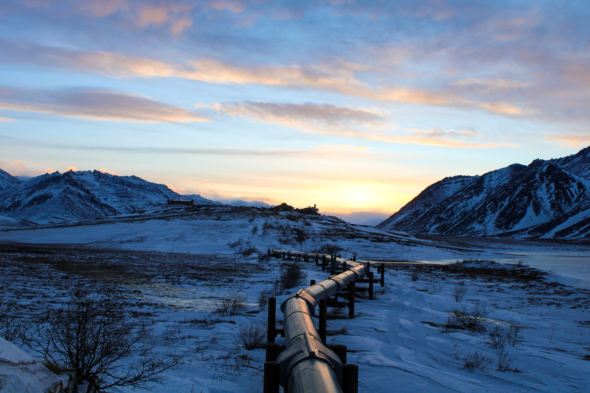
Management strategies in the tundra
- snake drilling: from one site, lateral drilling underground can reach more areas. This reduces the need for there to be infrastructure and heat pipes between oil extraction sites, which can melt permafrost and remove vegetation
- building on pads and piles: gravel pads absorb large amounts of heat, effectively replacing and complementing the active layer, reducing the heat the permafrost is exposed to. Spine Road, Prudhoe: 2m tall gravel pad.
- Piles are like stilts: infrastructure can be built on them, meaning that they are not in contact with the ground, using the air as a buffer between warm buildings and the permafrost.
- refrigerated supports: directly cools the ground below the infrastructure and the Alyeska pipeline, stopping the absorption of heat by the earth through direct cooling and creating a gap between the infrastructure and the ground
- supercomputers and AI: remote sensing and computation with the cloud and AI reduce the need for infrastructure to be built in areas to explore: predictions can be made accurately from afar.
Changes over time
3.a. Human factors can disturb and enhance the natural processes and stores in the water and carbon cycles.
3.b. The pathways and processes which control the cycling of water and carbon vary over time.
Equilibrium and Feedback Loops
The global carbon and hydrological cycles are typically in a state of dynamic equilibrium - a balance between all stores and flows in a system. This means that if there is an imbalance of one aspect of the system, such as the inputs, then processes and outputs will adjust to ensure that the system remains stable. In the long-term, this may be true. In the short term, the inputs, outputs and flows may sway from net gain to net loss, or vice versa, in disequilibrium. Negative feedback loops are examples of the system self-regulating. Positive feedback loops are the opposite.
Positive feedback loops
Positive feedback loops are a snowball effect. That is, the system, after a trigger occurs or threshold is reached, the system increasingly becomes out of balance.
In the water cycle:
- A greater greenhouse effect increases global temperatures. This means the atmosphere can hold more moisture. The higher temperatures increase evaporation rates. This increases the greenhouse effect. This means that temperatures are higher, and evaporation increases.
- Temperature increases in the atmosphere. This increases sea surface temperatures. This melts polar sea ice. This decreases the albedo effect from snow & ice cover. This increases sea surface temperatures…
In the carbon cycle:
- A greater greenhouse effect increases temps. Permafrost in the tundra is able to melt more quicky. CO2 and CH4 are released. This increases temperatures.
Negative feedback loops
In the water cycle:
- Higher temperatures from greenhouse effect. This increases evaporation. With more atmospheric water, more clouds are likely to form. This increases the albedo effect, reducing the amount of sunlight that is reflected as long-wave radiation. This lowers temperatures and evaporation.
- A rainfall event may occur. This increases the amount of infiltration and percolation into groundwater stores. The water table rises with more water. This increases overland flow, until the water level lowers. This lowers the amount of water in aquifers.
In the water cycle:
- Increased atmospheric CO2 emissions. This increases the amount of CO2 in the atmosphere. The CO2 available to plants increases, causing carbon fertilisation. Plants thus absorb more carbon from the atm. This lowers the atmospheric CO2 concentration.
Land use changes
A range of land use changes act as a catalyst for altering the flows and stores in the carbon and water cycles.
Urban growth
Urbanisation (change in land use from rural to urban). This:
-
replaces natural land with impermeable surfaces, such as tarmac;
-
reduce percolation and subsequent infiltration, increasing runoff;
-
encourage fast drainage of water after precipitation into sewage systems;
-
ultimately, decreasing the lag time and increasing peak flows.
-
decreases natural stores and sequestering of carbon, even releasing it from trees that may be burned;
-
requires additional surrounding land to sustain development, reducing diversity and carbon stores;
-
increases carbon emissions on a local scale from urban development and combustion.
Farming
Modern agricultural techniques require huge amounts of change to natural environments and huge amounts of water to sustain crop growth. In the Colorado River basin, USA, agriculture accounts for 80% of all water that is used.
- irrigation systems are typically located closest to rivers; reducing river flow and storage in aquifers
- irrigation increases water in the soil (pedosphere) temporarily, with an increase in evaporation and transpiration increasing relative humidity;
- aquifers may dry up, decreasing the local water table, lowering the number of springs, and flow in rivers.(could you link this to a negative feedback loop?);
- natural interception is reduced vs forest or grasslands;
- ploughing increases evaporation losses and decreases soil moisture;
- ditches and subsurface draining channel water rapidly away from being able to infiltrate and percolate, and into streams or gulleys, increasing peak flow;
- heavy machinery compacts areas of soil that inhibit infiltration on a local-scale
Forestry
Modifies the water cycle on a local scale, depending on the type of trees and area of effect.
Water Extraction
Water extraction includes surface extraction and also extraction of water from aquifers and artesian basins - thus the removal from these stores and transfer to others.
Artesian aquifers are those under artesian pressure. This means that in a syncline area - one confined by strata of impermeable rock geologies - water is able to travel to the surface, depending on the potentiometric surface. Imagine that the water table in an area of porous chalk is at the surface. However, the chalk in this basin - a U-shape with various layers of rock above and below - is at the base of this “U”. When drills are made into the bottom of this basin which may be above a population centre such as London, this water is able to rise to the surface, as a hole has been put into the impermeable rock.
In London, the water table fell by 90m due to industry. By 1990 it was recovering at 3m/yr. Underground infrastructure was threatened and Thames Water now has permits to abstract water, maintaining the equilibrium.
In the River Kennet, upstream from London, which drains 1,200 km2 of land, water extraction from sources has decreased river flow by 14% consistently. This is worse in droughts when up to 40% of the flow is lost. This reduces overland flow in the river, and also the flux as percolation into aquifers, whose water tables are less likely to rise to the surface, affecting a number of springs and saturated overland flow and water in surrounding areas. Water available for uptake by trees is also lost. Downstream, floodplains have seen a lowering in the water table and less time spent with the saturated ground.
How water and carbon are linked
4.a. The two cycles are linked and interdependent.
As I’ve hinted at and I’m sure you’ve realised by now, the water and carbon cycles are linked in many ways.
- Oceans
- Atmosphere
- Cryosphere
- Vegetation
Management strategies for carbon
At a local scale, an example of an all-round approach to management strategies can be seen with the UN’s REDD+ scheme - which offers incentives to companies and businesses to change the way forest resources are handled. “Carbon credits” can be purchased by TNCs from local tribespeople, who use the money for sustainable development with agroforestry and land stewardship, as opposed to more intensive agriculture, reducing emissions and deforestation. UNEP - REDD
Afforestation
Afforestation is the process of planting trees in areas where there are none, perhaps as a result of prior deforestation, or simply where trees do not traditionally grow. Trees need to have a permanence of 100 years to be an effective sink; they take up carbon in this period in the medium to long term. Over time, trees can absorb large quantities of C02 from the atmospheric store - around 1 tonne per tree.
The Chinese Great Green Wall and the one in Africa with the same name are examples of large-scale afforestation projects. An estimated 100 billion trees is being targeted to be planted by 2050 over a land area the size of Spain in the Gobi Desert, sequestering carbon (you can do the maths here) and also reducing desertification and land degradation - China’s biggest biological threat. The broader implications of afforestation may be a good idea to place in essay conclusions for 16-markers.
Of course, ensuring that the land does not become deforested in the first place, perhaps though legislation or policing against farmers and miners can be argued to be a more effective management strategy as this preserves the natural ecosystem. Or, legal but managed logging of areas that ensure that monocultures are avoided whilst preserving the biodiversity through the replanting of diverse trees may also be a better strategy.
Agricultural practices
Agricultural practices are also used in conjunction with afforestation, especially in areas previously subject to unsustainable practices or “slash and burn” techniques. Livestock farming, mostly cows, accounts for around 75% of deforestation in the Amazon, and emits over 100 million tonnes of methane, which is 28x more potent than just CO2, on top of the release of sequestered carbon in forest regions cleared for agriculture.
At a local scale, Degraded Land Afforestation in Uruguay uses “carbon financing” (carbon credits), which may come from REDD+, to plant trees on more degraded land, whilst cattle graze in the lower areas.
Indirect measures can also be taken: animal feed can be improved, such as by giving seaweed to cows reducing methane burp emissions by 82%. Manure can also be recycled or added to anaerobic containers can also be a way to generate energy in rural areas, reducing the reliance on fossil fuels.
Restoration of wetlands
Globally, wetlands account for around 7% of the land. But also 35% of the terrestrial carbon store - meaning that they are very effective carbon sinks. Compared to tropical rainforests, they can store up to 50x more carbon in the same area. Globally, peatlands store 2x more carbon than all forests.
The conditions of wetlands create low-oxygen soils, leading to anaerobic conditions. This inhibits the decomposition process and matter is thus unable to be broken down, accumulating as peat over time.
However, where these regions are widespread such as the tropics, human activity to sustain high population densities has reduced the amount of natural mangroves and salt marshes. Despite this reduction and associated risk to natural ecosystems, there have been schemes and actions taken to restore the prevalence of these wetlands. In Cambridgeshire, 500ha of low-lying land has been converted back to wetland as a result of the EU Habitats Directive. Controlled flooding of inland areas such as the Fens can also contribute to reclaiming land by the sea in these areas where the water table is naturally much higher.
In Canada, which is home to 25% of the world’s wetlands, 70% of the wetlands have been lost. However, pledges have been made to restore 30 percent of the degraded land by 2030 and over 1000 sq. km has been restored, sequestering almost 400,000 tonnes of C per year!
Carbon capture and storage
CCS is a technique used to stop carbon emissions from the source, such as in factories or power stations, or through directly capturing it from the air. Carbon dioxide may be captured and compressed, transported into a pipeline, and used in offshore oil extraction where otherwise it may be uneconomical to do so. Or, it could just be pumped into a syncline basin with impermeable rock where it remains hopefully for a long time.
International carbon agreements
The most effective way to protect the global carbon cycle may be international agreements. These provide a legal framework for large-scale, mass carbon emissions reductions globally, when done correctly.
1997 Kyoto Protocol
The Kyoto Protocol was the first major climate change protocol. Whilst it was legally binding, and 192 parties were included in it, many developing nations such as India and China - who “needed” to emit to continue their growth, were exempt from the protocol, and even some ACs such as the USA and Australia did not ratify the treaty. The overall goal of the protocol was to limit emissions to 5% of 1990 levels - and it worked. The protocol also had multiple rounds, the second of which capping emissions 18% below 1990 levels to 2020.
Kyoto introduced three major mechanisms to help reduce carbon (and the emission of other gases).
- Emissions trading: commoditises greenhouse gas emissions. Article 17 sets out the amount of greenhouse gas emissions that each country is permitted to emit, based on the overall target of the protocol (5% above 1997). Countries are allowed to buy and sell quotas of carbon - but due to supply and demand, prices of investing in sustainable development in the long term are cheaper. More details in the cap and trade section below.
- Clean development mechanism: This incentivises industrialised countries to invest in cleaner energy use in countries in the process of developing. This gives ACs flexibility on how quotas are reached - as the offset of carbon is counted as their emissions - whilst encouraging the use of these sustainable practices - such as the use of solar panels in rural communities - in developing nations. By 2012, this accounted for around 3 billion tonnes of CO2 reduction.
2015 Paris Climate Convention
The PCC in 2015 attempted to build on the successes of the Kyoto Protocol whilst also modernising it. It aims to limit CO2 emissions and temperature increase below 2 degrees C.
- Countries publish their naturally determined contributions and there is pressure at the global scale to consistently outperform other countries;
- Long-term strategies
Management strategies for water
There are global strategies that have the potential to protect the water cycle, including:
- forestry
- water allocations
- drainage basin planning
Forestry techniques
The protection of forests ensures that areas on a local scale are protected from deforestation in law. The UN, World Bank and governments all collaborate to ensure forests do not become degraded. The REDD+ programme funds projects in over 50 countries with direct investment, technology and carbon offsets.
NGOs such as WWF and the ARPA program in Brazil ensure that over 128 million acres of land, targeting 150 million, are protected.
Water allocations
In areas of water scarcity, water may be allocated by governments and rationed between different groups and stakeholders, such as businesses, farmers and individuals.
Agriculture, as seen in the Colorado River basin in the USA, accounts for over 80% of the water use. Globally agriculture accounts for over 90% of consumption, including municipal and industry sectors.
Management strategies:
- minimising water loss through evaporation with the use of drip irrigation, reducing usage by 70%.
- terracing and vegetative strips encourage the pooling of water on the surface. This reduces runoff and allows more time for water to infiltrate, moving through the soil as throughflow.
- capping usage for certain states (in the Colorado basin) to ensure that droughts do not disproportionally damage downstream states and environments.
Drainage basin planning
This is a collaborative effort at the drainage basin scale to encourage the sharing of demands and needs for everyone involved, including domestic use, industry and agriculture.
Calculations are made in relation to the amount and rates of fluxes in the system, with “targets” placed on stores. For example, stating that aquifers should always remain 50% at capacity with a high water table. After these plans have been made, actions can be taken, such as reforestation to improve interception rates, slowing peak flow, and encouraging greater infiltration and percolation. Urban areas can be financially incentivised to reduce the amount of impermeable surfaces - such as in the EU Water Directive Framework pre-2020 where 10 catchment hydrologies had holistic plans established to improve the amount and availability of water at this scale.
You’ve made it to the end of the content!
Good luck with your exams!
Feel free to share this Cheat Sheet with friends, family and teachers.
If you found this useful, please do send a message on Discord to let me know! This document has over 18,000 words hand-written by me, all available for free, so messages are appreciated :)
Made with 💕 by Draggie
Paper 1 - Additional Skills
The OCR specification also lists some specific skills you must have to ensure you get full marks. These topic-specific skills are:
- climate graphs
- simple mass balance (remember from glaciation?)
- rates of flow
- unit conversions
- analysis and presentation of field data
Statistical tests
Median
Rank the data and work out the middle value. If it’s between two points, then take the mean value between them.
- easy to calculate
- not affected by extreme, anomalous values
- most of the values are ignored
- less “sensitive” than the mean (a significant change on one side can be balanced by a small number on the other)
Mean
Add all values in the series together and divide by the total number of values. This is the “average”.
- all values accounted for
- gives fair representation for all values
- affected by all values even if anomalous/very large or small.
Mode
The value that occurs in data the most.
- can be used on qualitative data
- useful for spotting patterns
- may be multiple modes, or none at all
- only useful for specific enquires
Range
Subtract the lowest from the highest value in the data.
- shows the full spectrum of all data
- can be significantly affected by extreme values
- most data is ignored
Interquartile range
Rank the data, then identify the median. For all values below the overall median, calculate the median. Repeat for the upper half. Then, subtract the lower half median from the upper half median.
- measures dispersion of data
- not easily affected by outliers
- doesn’t include all values
Spearman’s Rank
Tests the significance of a correlation between two variables.
Compare the number of items (degrees of freedom) given to the significance table. The hypothesis can be rejected if the number in the table is below the critical value at 0.95, then your hypothesis can be rejected. If it’s above, then there is less than a 5% that the relationship was caused by chance, and you accept the hypothesis. You can go even further if given a critical value of 0.99, which means there is a less than 1% chance of this being caused by chance!
If you have a t-value, then subtract 2 from the degrees of freedom. Else, leave it as the number of samples.
Confidence intervals can be obtained from the following formula:
(no need to know this - unless you do maths?)
THE END